
Regression is a statistical methodology that describes the relationships between a continuous explained variable and a set of explanatory variables. In other words, regression models are able to predict the value of a dependent variable y with respect to a set of ![]()
![]() independent variables
independent variables ![]() .
.
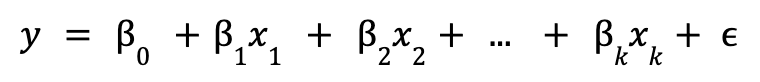
Linear regression is a regression model where the relationship to be explained is linear. This characteristic makes the models easy to interpret, but at the same time it can be restrictive when the relationships are more complex. The population linear regression model is defined as:
where ![]()
![]() is the intercept,
is the intercept, ![]() are the model parameters and
are the model parameters and ![]() is the unobservable error term, which represents the factors other than
is the unobservable error term, which represents the factors other than ![]() that affect
that affect ![]() .
.
When to use linear regression
The linear regression model should be used when looking to create a simple and fast model, as no hyperparameters need to be fitted. Part of the simplicity of the model comes from the linearity of the terms. This may seem like a major restriction, but in reality linearity should only exist between the dependent variable ![]()
![]() and the parameters of the model
and the parameters of the model ![]() , not with the independent variables
, not with the independent variables ![]() .
.
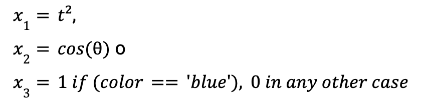
This means that independent variables such as the following could be valid to build the model.
It is also advisable to use linear regression when interpretability is prioritised over performance or results, as each parameter of the model allows us to understand what the weight or effect of the variable in question is on the explained variable while holding all other explanatory variables constant.
In terms of variables, the explained variable is expected to be numerical. If the dependent variable is categorical rather than numerical, a classification model, such as a decision tree, should be sought. If the dependent variable is binary categorical, a logistic regression can be used to model the probability of a category.
Additionally, the explanatory variables should not show high multicollinearity, that is, they should not be able to be expressed as a combination of other variables used in the model.
Ordinary least squares method
Once the population linear regression model is established, a methodology is needed to obtain its parameters. However, one usually does not have data from an entire population, but from a small sample of data. Consequently, estimates of these parameters must be obtained from the sample to see if they approximate the population parameters. The branch of statistics that deals with drawing conclusions about population properties from a sample is called inferential statistics.
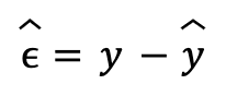
The ordinary least squares (OLS) method states that the best estimators for linear regression parameters are those that minimize the sum of squares of the residuals. Residuals are defined as the difference between the actual value of the explained variable and the value predicted by the model:
The result of this minimization allows us to arrive at a mathematical solution for the parameter estimators without the need to use numerical optimization, that is, the estimators can be calculated with formulas from the data. This is not necessarily the case with other residual minimization functions. The resulting formula in matrix form is:

where the matrix of independent variables ![]()
![]() has dimensions of k+1 (k variables and the constant term) and m observations, the vector of dependent variables Y has dimensions of m observations and the estimators of the linear regression parameters
has dimensions of k+1 (k variables and the constant term) and m observations, the vector of dependent variables Y has dimensions of m observations and the estimators of the linear regression parameters ![]() have dimensions of k+1 variables (k variables and the constant term). The same result can be obtained from assuming that the unobservable error term has zero mean and is uncorrelated with the explanatory variables.
have dimensions of k+1 variables (k variables and the constant term). The same result can be obtained from assuming that the unobservable error term has zero mean and is uncorrelated with the explanatory variables.
Interpreting the results
The ordinary least squares method provides a way to obtain parameter estimators for a linear regression model. However, ways are needed to measure the performance of the model and its predictions and to be able to compare it with others.
One way may be to again use the sum of the square of the residuals. By comparing this metric in two models predicting the same explained variable, one can determine which of the two models best predicts the value of the explained variable by choosing the one with the smaller error. In many cases, a square root is applied to this metric to maintain the same units as the explained variable.
In other cases, it is more interesting to have a metric that is unitless. This is the case for the coefficient of determination ![]()
![]() . Values of this coefficient close to 1 imply that the predicted
. Values of this coefficient close to 1 imply that the predicted ![]() values are close to the true
values are close to the true ![]() value, while values close to 0 indicate that little variation of the true
value, while values close to 0 indicate that little variation of the true ![]() value is captured by the variation of the predicted
value is captured by the variation of the predicted ![]() value.
value.
The outcome of the metrics seen establishes how good the predictions of the model are. However, as a general rule, as more explanatory variables are added to the model, these metrics show better results, regardless of whether or not the variables are part of the population model. When you want to determine whether the model created from the sample data correctly describes the population model, you have to turn to inferential statistics and hypothesis testing.
In hypothesis testing, one establishes a null hypothesis ![]()
![]() about a population parameter and tries to contradict it with sample data. In practice, a probability threshold or α significance level is set and the probability of obtaining a value of the sample estimator equal to or more extreme than the null hypothesis is calculated. This probability is called the p-value and when this is less than the significance level, it is decided to reject the null hypothesis, assuming that rejecting it will be wrong in α% of the cases.
about a population parameter and tries to contradict it with sample data. In practice, a probability threshold or α significance level is set and the probability of obtaining a value of the sample estimator equal to or more extreme than the null hypothesis is calculated. This probability is called the p-value and when this is less than the significance level, it is decided to reject the null hypothesis, assuming that rejecting it will be wrong in α% of the cases.
In the case of linear regression, tests of ![]()
![]() can be performed to determine whether, individually, the
can be performed to determine whether, individually, the ![]() estimators are statistically significant and to assert that the variable
estimators are statistically significant and to assert that the variable ![]() is relevant to predict
is relevant to predict ![]() , that is, that
, that is, that ![]() is different from zero. In a similar way,
is different from zero. In a similar way, ![]() tests can be performed to determine whether, jointly, several or all of the parameters are significant.
tests can be performed to determine whether, jointly, several or all of the parameters are significant.
These tests are useful to determine whether some explanatory variables should be discarded, even though they may contribute value in the variance explained. In other words, they help to avoid overfitting the model to the data. On the other hand, when relevant variables are omitted from the model, a bias is produced in the rest of the estimators (underfitting).
Examples in Python
In the following, we will see how to create linear regression models in Python using two different libraries. First, the Scikit-learn (sklearn) library provides a multitude of tools for creating, fitting and evaluating machine learning models. It provides a multitude of regression, classification, clustering, etc. models. Among the tools included in this library are methods for preprocessing data, tools for selecting the best model and facilitating the adjustment of hyperparameters or the reduction of the dimensionality of the input data.
Using the Scikit-learn library is very simple, since the use of many of its tools follows the same scheme: the required class (for example, a model) is instantiated by setting some parameters, it is adjusted to the data using the fit() method and, finally, the adjustment is executed on the data using predict() or transform() depending on whether a model has been adjusted or a transformation is desired. The model parameters can be found in the attributes of the model once it has been fitted.
In the following example, a linear regression model is created in Scikit-learn for previously generated data, consisting of 3 explanatory variables and one explained variable, with a total of 30 records. First, the data is loaded into a DataFrame from the pandas library.
import pandas as pd
df = pd.read_csv('data.csv')
print(f"Filas: {df.shape[0]}")
print(f"Columnas: {df.shape[1]}")
df.head(5)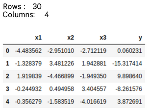
Next, the LinearRegression class is used to create and fit the linear regression model. The estimators of the regression parameters are displayed by accessing the intercept_ and coef_ attributes of the fitted model.
from sklearn.linear_model import LinearRegression

X = df[['x1','x2','x3']]
Y = df.y

lr = LinearRegression()
lr.fit(X, Y)

print(f'b0 = {lr.intercept_:7.4f}')
print(f'b1 = {lr.coef_[0]:7.4f}')
print(f'b2 = {lr.coef_[1]:7.4f}')
print(f'b3 = {lr.coef_[2]:7.4f}')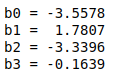
Finally, the model is evaluated using different metrics from sklearn.metrics. A high value of the coefficient of determination is obtained. This implies that the predictions obtained are fairly well adjusted to the real values.
from sklearn.metrics import mean_squared_error, r2_score
Y_pred = lr.predict(X)

print(f"MSE  = {mean_squared_error(Y, Y_pred):6.3f}")
print(f"RMSE = {mean_squared_error(Y, Y_pred, squared=False):6.3f}")
print(f"R2   = {r2_score(Y, Y_pred):6.3f}")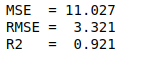
On the other hand, the Statsmodels library provides a multitude of models and statistical tests on which to test the data. To fit a linear regression, the OLS class is used. After fitting the data with the fit() method, the results can be displayed in a very detailed way using summary(). Next, a fit is performed with this library using the same data as before.
import statsmodels.api as sm

X = df[['x1','x2','x3']]
Y = df.y

# Se añade una variable constante de 1 (b0*1)
# A constant variable of 1 (b0*1) is added
X = sm.add_constant(X)

ols = sm.OLS(Y, X)
results = ols.fit()

results.summary()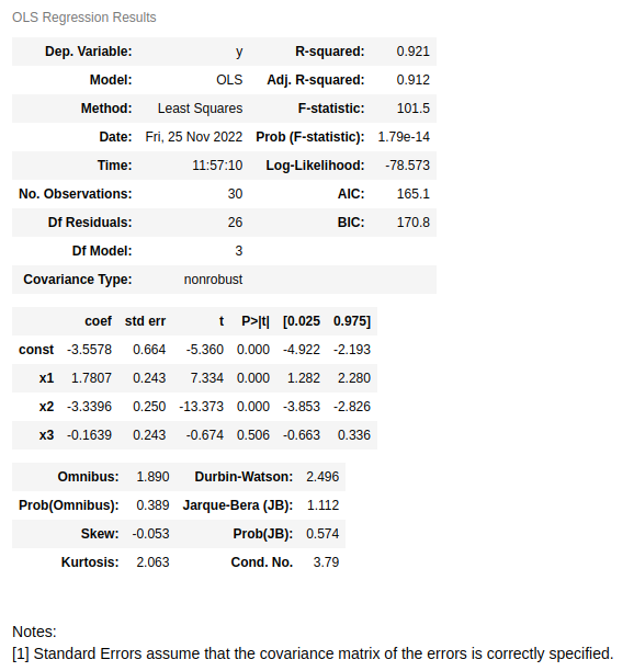
In the first table of the results it can be seen that the same value of ![]()
![]() is recovered and in the second table it can be seen that the estimators also coincide. Additionally, in the above table the value of the
is recovered and in the second table it can be seen that the estimators also coincide. Additionally, in the above table the value of the ![]() statistic and the p-value of the test of
statistic and the p-value of the test of ![]() are also plotted. In this case, this test sets as a null hypothesis that all parameters used in the regression are zero and do not help to explain the dependent variable. The resulting value is very small and, therefore, the null hypothesis is rejected, that is, there is some variable chosen in the model that does have weight in explaining
are also plotted. In this case, this test sets as a null hypothesis that all parameters used in the regression are zero and do not help to explain the dependent variable. The resulting value is very small and, therefore, the null hypothesis is rejected, that is, there is some variable chosen in the model that does have weight in explaining ![]() .
.
On the other hand, the second table, to the right of the values of the estimators, shows the error associated with each one, the value of the ![]()
![]() statistic, the p-value obtained from performing the
statistic, the p-value obtained from performing the ![]() test and the confidence interval of each estimator of 95% (α=5%). It can be seen that the p-value for the
test and the confidence interval of each estimator of 95% (α=5%). It can be seen that the p-value for the ![]() variable is high, compared to the typical probability threshold (5%). This means that
variable is high, compared to the typical probability threshold (5%). This means that ![]() cannot be said to be non-zero. In other words, there is not enough statistical evidence in the sample to reject the null hypothesis of the test of
cannot be said to be non-zero. In other words, there is not enough statistical evidence in the sample to reject the null hypothesis of the test of ![]() performed on this parameter. Therefore, it might be appropriate not to use it in the model.
performed on this parameter. Therefore, it might be appropriate not to use it in the model.
Conclusion
In conclusion, linear regression is a simple model that allows explaining the values of a numerical variable as a linear combination of different explanatory variables. The ordinary least squares method allows estimating population parameters, which can be interpreted as the weight of the independent variable on the dependent variable. Tests can be performed on these estimators to understand whether the model created from a sample is adequate to explain the population.
Finally, two possibilities for implementing linear regression in Python have been explored. The Scikit-learn and statsmodels libraries have been used. The former is oriented towards machine learning, with a multitude of tools and models to process the data, while the latter is oriented towards statistics, with different hypothesis tests to test the data.
So much for our post of the day. If you found it interesting, we encourage you to visit the Data Science category to see more articles like this one and to share it with all your contacts.
