The linear regression model is one of the most useful tools in every data scientist’s kit bag. Although this post is geared towards people with first-hand knowledge of this statistical model, it never hurts to remember that linear regression aims to predict a quantitative variable response y (also known as the dependent variable) as a linear combination of a set of predictors x1, x2, …, xk (also known as independent variables, explanatory variables or predictors).
With this motivation, the linear regression model introduces a series of coefficients or population parameters that represent the relationship of each predictor with the response variable, resulting in the classic equation that we all have seen represented at one time or another.

These population parameters are estimated from a dataset using the ordinary least squares (OLS) method, which guarantees under a set of assumptions (Gauss-Markov assumptions) that the statistical estimators of these parameters are unbiased. Among these assumptions, there is one known as additional, the homoscedasticity assumption, which is necessary to be able to make inference from the regression coefficients, something that can be of great value in certain contexts.
In this article, we are going to talk about this last additional assumption, commenting on the impact of not complying with it when interpreting the coefficients of a regression, providing tools to detect whether this assumption is being fulfilled and offering solutions to solve real use cases in which this assumption is not satisfied.
Before proceeding with the reading of the article, it is recommended to take a look at the appendix defined at the end of this one, since it contains several definitions that will be essential to be able to follow and to understand all the content to be developed.
What is heteroscedasticity?
In the linear regression equation presented in the introduction, we can appreciate a last concept commonly referred to as the unobserved error term, which represents those factors independent of the predictors that affect the response variable y.
Once this unobserved error is defined, we say that, in the framework of linear regression, a model presents homoscedasticity when given any value of the explanatory variables the variance of the unobserved error remains constant. On the other hand, we speak of heteroscedasticity when the variance of the unobservable error varies for different segments of the population, where these segments are characterized by different values of the predictors.
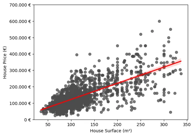
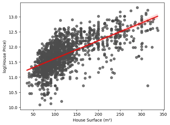
A simple scenario in which this phenomenon can be observed is in a simple linear regression model in which the price of housing is modeled as a function of a single explanatory variable: square footage. As we can see in the following graph, it is clear how the variance of the errors with respect to the fitted regression is not constant, being notably higher for those cases in which the surface area is larger.
Impact of Heteroscedasticity in Linear Regression
Heteroscedasticity can have a large impact on the inferences made from our regression. This is mainly due to the additional assumption we discussed in the introduction for estimating the population parameters of the model with OLS, which states that the model must not exhibit heteroscedasticity. In other words, the unobserved error variance is required to remain constant with respect to the explanatory variables. So, why is this assumption necessary and what are the implications of not satisfying it?
Knowing why the assumptions of linear regression are necessary is not a trivial task and is beyond the scope of this post, but we will still give a couple of hints so the reader can quantify the importance of respecting the assumption of constant variance of the unobserved error.
So far, we have called this assumption an additional assumption, and this is because the homoscedasticity assumption is not necessary to conclude that the estimators produced by the OLS method are unbiased. At this point, some may be asking the following question: If heteroscedasticity does not cause bias or inconsistency in OLS estimators, why is it introduced as an assumption? In short, this assumption brings us several benefits over those that are strictly necessary to prove that OLS estimators are unbiased:
- Imposing this assumption greatly simplifies the mathematical development necessary to apply the OLS method.
- The OLS method acquires an important efficiency property, that is, the variance of the estimators of the population parameters is lower when this assumption is introduced.
- It allows us to define unbiased estimators of the sampling variance of the population parameter estimators.
The most important of these three benefits is the last one mentioned, since without the assumption of heteroscedasticity the variance estimators are biased. The standard errors of the parameters estimated by OLS are based directly on this variance, so if this assumption is not satisfied, these errors are no longer valid for the construction of confidence intervals and statistics used in classical hypothesis testing. As a final conclusion, this assumption is key to perform statistical inference on the underlying population model from a data sample, since the usual OLS inference is incorrect in the presence of heteroscedasticity.
How to detect whether heteroscedasticity exists?
Although, as we have seen, heteroscedasticity can be a problem, there are several statistical tests that allow us to detect it in a simple way. In this post, we are going to see one of these tests in detail, showing the fundamentals on which it is based.
Breusch-Pagan test
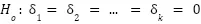
The Breusch-Pagan test for heteroscedasticity arises from the idea of posing the null hypothesis (the error variance is constant given the values of the explanatory variables) as a new regression adjustment. This new regression model considers the unobserved squared error as the dependent variable, and the same explanatory variables as the original model. This way, the previously stated hypothesis to be rejected can be represented as the following:

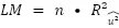
We will never know the actual errors of the underlying population model, but we can obtain a good estimate of them from the OLS residuals. Finally, the LM statistic to be used to test the hypothesis will be specified by the sample size and the goodness of fit of the model with the squared residuals as the dependent variable.
In summary, the procedure to carry out this test is as follows:
- Estimate the OLS regression model in normal form, in order to obtain the squared residuals.
- Fit the regression in which the independent variable is the squared residuals previously obtained, and the explanatory variables are the same as those of the original model.
- Calculate the R-squared of this second regression.
- Calculate the statistic from the multiplication of the sample size and the R-squared previously obtained.
- Using the Xi distribution with as many degrees of freedom as explanatory variables in the model, calculate the p-value in order to determine whether, with a chosen significance level, the null hypothesis of homoscedasticity previously stated is rejected.
Other tests for heteroscedasticity
As we have already mentioned, there are other tests that allow us to detect heteroscedasticity. In these cases, their names are only mentioned to give the reader the ability to investigate in more detail the differences between them:
- White’s test
- Bartlett’s test
- Goldfeld-Quandt test
- Park’s test
Solutions to the heteroscedasticity problem
There are several ways to solve this problem when inference is intended. In this post, three possible solutions will be presented, describing in brief what they consist of.
Robust inference
Although in the presence of heteroscedasticity classical inference using OLS estimation is invalid, this does not imply that OLS estimation is useless for inference in this type of scenario. It is possible to adjust the standard errors, and, by extension, the different statistics classically used in inference, so that they are useful in scenarios in which heteroskedasticity exists even if neither the behavior nor the form of such heteroskedasticity is known. It is beyond the scope of this article to explain the mathematical deduction behind these adjustments, since it presupposes a fairly strong background in statistics.
This adjusted standard error is known as robust standard error to heteroscedasticity, although in the literature it also appears as White’s, Huber’s or Eicker’s standard errors. From this robust standard error, it is possible to construct a t statistic and an F statistic robust to heteroscedasticity. Most statistical packages have utilities to calculate the robust version of the statistics and make life easier for the user.
It should be noted that these robust versions of the statistics are only suitable for inference if the sample size is large enough, since with small sample sizes it may happen that their distributions differ significantly from the distribution to which the non-robust version of the statistic tends, making the inference invalid. It is for this reason that classical statistics are usually preferred to be used at all times, except in scenarios where there is clear evidence of heteroscedasticity.
Weighted least squares adjustment
There are scenarios in which the shape of the heteroscedasticity is known in advance, so it is possible to specify that shape and obtain an estimate by the weighted least squares method (OLS). In case the form of heteroscedasticity has been correctly specified, the MCP method is more efficient than OLS, and leads to valid statistics for making inference with correct distributions.
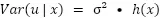
To specify the heteroscedasticity, a function h(x) is introduced that varies the variance as a function of the explanatory variables. Given this, we can, for example, define that this function is equivalent to the value of one of the explanatory variables of our model, making the error variance proportional to the value of that variable.
Introducing such a strong assumption as assuming that the form of the heteroscedasticity is known begs the question: what happens if the form is misspecified? In this scenario, one can be assured that the estimators returned by MCP remain unbiased and consistent, although there are two consequences of this misspecification:
- The standard error and statistics are no longer valid for inference, even in cases where the sample size is large. Fortunately, it is possible to obtain standard errors robust to arbitrary heteroscedasticity for MCP in a manner similar to what we have previously discussed with OLS.
- There is no guarantee that MCP is more efficient than OLS. This fact, although theoretically true, has no significant practical importance.
In general, in cases where there is strong heteroscedasticity, it is usually more convenient to specify an incorrect form of heteroscedasticity and use OLS than to ignore it completely and use OLS.
Dependent variable transformation
A possible simpler and more practical solution to this problem is to transform the response variable y using a concave function, such as the natural logarithm function log(y). This type of transformation greatly reduces those values of the independent variable that are larger, leading to a reduction in heteroscedasticity.
The following image shows how the graph previously shown would look like to explain the heteroscedasticity in the case of transforming the dependent variable. As can be seen, the variance of the residuals appears to be more constant than it was previously.
It is important to emphasize that these types of transformations cause a complete change in the interpretation of the regression coefficients.
Conclusion
In summary, heteroscedasticity is a threat when making statistical inference from a linear regression model fitted by the ordinary least squares method. However, thanks to this article, you are now prepared to detect this phenomenon so that you can act accordingly to mitigate its impact on your statistical analysis.
Appendix
In this appendix you will find several relevant concepts in order to understand all the details of this post.
Population parameter: A numerical value that describes a specific characteristic of a complete statistical population. This type of value is usually unknown, so it is estimated from a population sample.
Statistical estimator: A quantitative measure derived from a population sample used to estimate an unknown parameter of that population.
Bias: We can define bias as the difference between the average or expected value of an estimate and the true value it is intended to estimate. If an estimator is biased, it will tend to systematically overestimate or underestimate a population parameter.
Variance: A measure used to quantify the dispersion of a random variable with respect to its average value. In other words, it measures on average how far the values of a random variable are from their expected value.
Consistency: Characteristic of a statistical estimator that indicates that, as we increase the size of the sample used, it is increasingly less likely that the estimator obtained is far from the true value of the population parameter to be estimated.
Efficiency: Given two unbiased statistical estimators, one estimator is said to be more efficient than the other when its variance is equal or smaller for any population parameter.
If you found this article interesting, we encourage you to visit the Data Science category to see other posts similar to this one and to share it on social networks. See you soon!
