
Nowadays, when talking about neural network models, it is common to mention how many graphics cards they need. For larger ones, there is talk of how many cards are needed, and how many GB of RAM may be required for a graphics card, for smaller ones. But it is rarely questioned why exactly the graphics card is the tool of choice. After all, not so long ago, it was limited to graphics-related calculations, not machine learning.
Therefore, in this post, we will show an overview of the graphics card architecture and an example of a graphics card accelerated operation to demonstrate its use. Because an example is programmed in this article using CUDA, everything mentioned is specifically about NVIDIA graphics cards, even if the concepts are applicable to other cards.
Architecture at a glance
To understand the architecture, it is important to first understand its major difference from a classical CPU. A classical CPU executes in a SISD (Single Instruction Single Data) architecture, that is, a single stream of instructions executes on a single stream of data. This means that there is only one program counter per processor and the processor can only load one data at a time.
On graphics cards, on the other hand, we find SIMT (Single Instruction Multiple Threads), that is, multiple processors are fed by a single program counter. In practice, this means that a group of processors execute the same instruction stream on one data stream each.
This difference means that, by its very architecture, the graph is massively parallel and this parallelism is the basis of the efficiency of the graph. This can be seen in the number of “processors” a graphics card has compared to a CPU. For example, the NVIDIA A100, a very popular graphics card for machine learning, has 6912 processors.
But, it is a limited parallelism, not every task that can be divided into subtasks can make use of this architecture, since, due to the SIMT model, a simple “if” can slow down the process considerably.
Resource management
The resources mentioned above cannot be accessed directly, an API is needed to expose them. In this case, we will talk about CUDA and how it exposes computational resources to the programmer.
Threads are the most essential unit. Each thread is a set of instructions to be executed and runs on one and only one processor (CUDA core). Above the threads are thread blocks, which are conceptually a grouping of threads that must not exceed a limit number (depending on the card, the figure is usually 1024). In addition, they have a small amount of shared memory between all threads belonging to the block and it is possible to synchronize the threads in the same block.
Finally, there are the kernel grids, which organize the blocks but do not share anything between them except main memory, and cannot even synchronize with each other. In this way, it is possible to call the required number of threads using a grid of thread blocks.
The lack of any synchronization resources outside the block level means that parallelism has to exhibit a property in order to make use of the graph, it has to be task parallel. Ideally, we would want it to be an instruction set that has to be executed on all data, and it is always the same instruction set. This limits the number of operations available, but there is one operation that is the basis of modern neural networks that benefits greatly from this type of parallelism: matrix multiplication.
Short example
To show the effect of running an operation on graph, we will compare it with the same operation on CPU using the sklearn implementation. All the code is available on Damavis’ GitHub.
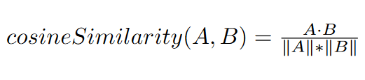
The example will consist of computing all cosine similarity between a 300-element vector and 2.2 million 300-element vectors, specifically, the entire GloVe word embedding model.
First of all, it is necessary to define the kernel, the function to be executed on the graphics card, which is done in CUDA, which is very similar to C as a language.
__global__ void cosineSimilarity (const unsigned int limit, const float* A, float* distanceOut,float* C_model, const float normA) {The kernel definition, requires limit, which indicates how many operations we compute, because due to the way specifying threads works, it is very common to have more threads than data. In this case, it is normal to ignore these extra threads.
The kernel also requires the vector A, against which we compute the cosine similarity; distanceOut, where we send the result of the operation; C_model, where we store all the vectors; and normA, which is the L2 norm of A.
__shared__ float fastA[300];This is the shared memory between blocks of threads that we mentioned previously. This memory is fast access, as it is the equivalent of the L1-level cache, the smallest and fastest cache on the CPU, except that it is explicitly managed by the user.
const unsigned int id = blockIdx.x * blockDim.x + threadIdx.x;
if (threadIdx.x < 300) {
	fastA[threadIdx.x] = A[threadIdx.x]; // only one embeding is on A
}
We load vector A into shared memory, since A will be read in its entirety by multiple threads, making it a good candidate for this one. Since we cannot be sure that the threads that have loaded the vector into memory are synchronised, we force a synchronisation with __syncthreads(), otherwise they might try to read data that is not yet loaded.
if (id < limit) {
	float acum = 0;
	float c_norm = 0;
	const unsigned int row = id / 8; // Get row
	const unsigned int interiorId = threadIdx.x % 8;  // Get id within row
	for (unsigned int i = interiorId; i < 300; i += 8) {
    	float cvalAux = C_model[row*300+i];
    	acum += fastA[i]*cvalAux; // Accumulate within the accumulator
    	c_norm += cvalAux*cvalAux;
	}
	acum += __shfl_down_sync(0xffffffff, acum, 4); // Reduction
	acum += __shfl_down_sync(0xffffffff, acum, 2); // Reduction
	acum += __shfl_down_sync(0xffffffff, acum, 1); // Reduction

	c_norm += __shfl_down_sync(0xffffffff, c_norm, 4);
	c_norm += __shfl_down_sync(0xffffffff, c_norm, 2);
	c_norm += __shfl_down_sync(0xffffffff, c_norm, 1);
We compute the inner product and the L2 norm, only using the threads that are below the limit. To make better use of the memory bandwidth of the graphics card, we make multiple threads work on a single inner product, specifically, eight. Generally, due to the memory architecture, this will give better results, so it is, in general, better to read with stride and not sequentially if possible in order to make better use of the available resources.
Finally, it accumulates the values of all eight threads into one, using the __shfl_down_sync() function. This allows sharing data between threads belonging to the same SM (Streaming Multiprocessor). We won’t go into what an SM is, but, in short, blocks of threads are executed by SMs, and an SM usually consists of 32 threads. But we won’t explain more in this blog post, as it requires more advanced knowledge of the architecture but it is not necessary, as you could do this same shrinking operation on shared memory.
if (interiorId == 0) { // Final step and write results
   	float simVal=(acum / (normA * sqrtf(c_norm)));
   	distanceOut[row] = simVal;
   	}
  }
}
Because we only compute a cosine similarity for 8 threads, we only write the result if it is the thread relegated to it. In this case, if it is a multiple of 8, it is the relegated thread.
Once we have the kernel defined, it remains to run it from python to do our test against sklearn. We use pyCUDA for this.
c_model_gpu = cuda.mem_alloc(embeddings.nbytes)
grid_dot = ((rows // 64) + 1, 1)
block_dot = (512, 1, 1)
cosine_similarity.prepare(("I", "P", "P", "P","F"))
a_gpu = cuda.mem_alloc(300*4)
distances_gpu = cuda.mem_alloc(rows*4)
norm=numpy.linalg.norm(word)
cuda.memcpy_htod(a_gpu, word)
cosine_similarity.prepared_call(grid_dot, block_dot, rows * 8, a_gpu, distances_gpu, c_model_gpu,norm)
cuda.memcpy_dtoh(final_result,distances_gpu)
Running the kernel against sklearn’s implementation of cosine similarity, – sklearn.metrics.pairwise.cosine_similarity – about 100 times, we get almost 70 times faster speedup, using the “NVIDIA GeForce GTX 1650 Mobile” graphics card with 1024 processors against the “Intel(R) Core(TM) i7-9750H” CPU. Both are relatively weak pieces of hardware in the deep-learning world, but especially the graphics card is the weaker piece.
| CPU | GPU | |
| Average time | 2.131s | 0.0278s |
| Standard deviation | 0.303s | 0.000269s |
| Speedup on CPU | 1 | 76.74 |
Conclusion
In summary, the graphics card is used because in the specific workloads required for deep-learning, its execution model is extremely appropriate, rather than that of the CPU itself, and this is because graphics cards have been trying to deal with the problem of how to make matrix multiplication more efficient since their inception. This allows graphics cards to achieve massive speedups when compared to CPUs.
So much for today’s post. If you found it interesting, we invite you to visit the Algorithms category to see other similar articles and to share it in networks with your contacts. See you soon!
