
What is a linear regression?
A linear regression is a model that is used to approximate the linear relationship between a dependent variable Y and a set of independent variables X. In matrix format it can be expressed as
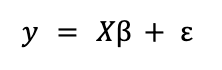
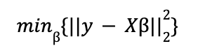
where ε is a vector of random terms or errors. β is that of the parameters to be estimated, a process that is carried out by solving an optimization problem in which the objective is to minimize the mean squared error (MSE). That is, by applying the ordinary least squares (OLS) method.
For an in-depth look at linear regression, read the post on Linear Regression with Python on our blog.
OLS is a method that has not lost its relevance since Gauss started using it in the early 19th century, although, as Hasties, Tibshirani & Wainwright (2015) point out there are two reasons why alternatives might be considered:
- Prediction accuracy can sometimes be improved by decreasing the value of the regression coefficients. In this sense, reducing the value of the estimators increases the bias but reduces the variance in the values to be predicted.
- According to the first point, the coefficients can be reduced to zero by selecting variables indirectly. In a model with a large number of explanatory variables at the beginning, it improves its interpretability.
Lasso and Ridge are two methods that combine the minimization of the OLS mean square error with the establishment of limits or penalties to the coefficients.
Definition of penalties L1 and L2
Lasso (L1) penalizes the sum of the absolute value of the coefficients. In this case, the minimization function in Lagrangian form would have the form

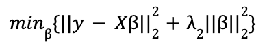
Ridge (L2) penalizes the sum of the square of the coefficients. The minimization function in Lagrangian form is:
where, in each case, λ represents the fitting parameter with value ![]()
![]() .
.
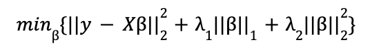
The combination of both penalties is the expression of an Elastic Net:
Although formally, and also in the Scikit-Learn and Statsmodels implementations, the expression that is minimized is slightly different:
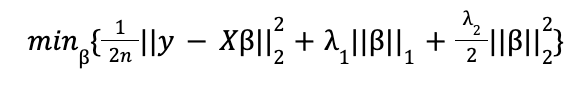
where n is the sample size.
Regarding the L1 and L2 penalties, it should be noted that:
- Compared to the OLS solution, both methods reduce the value of the coefficients, but only the L1 penalty can make some of them zero. Therefore, L2 is not suitable for automatic variable selection.
- If there are highly correlated variables, L1 could randomly choose one of them and set the other as zero.
- Since L2 does not cancel coefficients, the coefficients it returns are better distributed. In some cases it may be preferable to L1 if the model does not have many explanatory variables and it is certain that all of them should be in it.
- In both cases, different values of λ (img07) may be associated with different levels of bias and variance. The optimal point in the trade off between these two measures is the one that would minimize the Mean Squared Error (MSE).
- In any case, as a priori both methods consider the coefficients jointly, it is important to rescale the variables before running the regression. Otherwise, the coefficients of variables in different ranges would be regularized with the same criterion.
The Python implementations for the Elastic Net, whose extreme cases include the Ridge and Lasso regressions, are discussed below.
Linear regression with elastic net in Python
As an example, the load_diabetes package from sklearn.datasets, divided into training and test data, will be used.
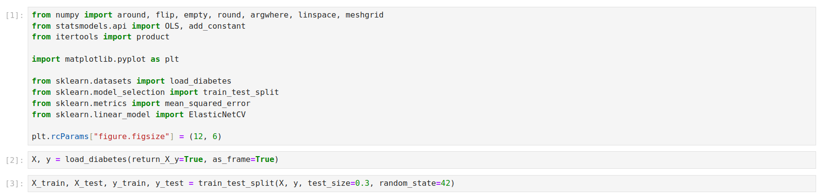
The data are already standardized.
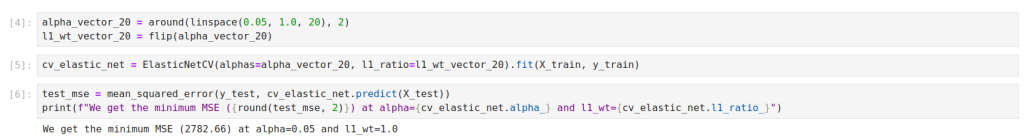
Scikit-Learn
In scikit-learn, linear regressions with elastic net can be performed with the ElasticNet and ElasticNetCV classes. Regularization is applied with the parameters alpha(s) and l1_ratio passed to the class. alpha(s) is the value representing the joint severity of the fitting parameter; l1_ratio is a value between 0 and 1 representing the proportion of L1 over the total penalty. ElasticNetCV supports vectors for alphas and l1_ratio and the best model is selected automatically.
Note, however, that the values in alphas and l1_ratio do not correspond to the penalties λ1 and λ2 of the elastic net as defined in Equation 6. As the package documentation itself points out in the ElasticNet class, if one wanted to control the penalties independently, one could consider that, for each combination of values in alphas and l1_ratio:
alpha = λ1 + λ2
l1_ratio = λ1 / (λ1 + λ2)
Thus, with given values of λ1 and λ2, the values should be translated into alphas and l1_ratio before passing them to ElasticNetCV.
Some useful parameters with which to test alternatives include fit_intercept=False and positive=True which, respectively, can be used to run regressions with no intercept or forcing a positive value on all coefficients.
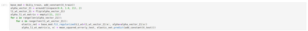
Statsmodels implementation
In Statsmodels, the regularization is applied with the parameters alpha and L1_wt within the .fit_regularized method. As with scikit-learn, for Elastic Networks, the alpha penalty is split between both regularizations depending on the value of L1_wt, equivalent to l1_ratio in scikit-learn.
Statsmodels does not allow direct cross-validation. Although it would be possible to apply it with further development, it is obviated because it is beyond the scope intended here. In Statsmodels, testing different values of alpha and L1_wt requires running loop regressions to choose the best combination.
Representing the alpha – L1_wt value matrix in a heat map:
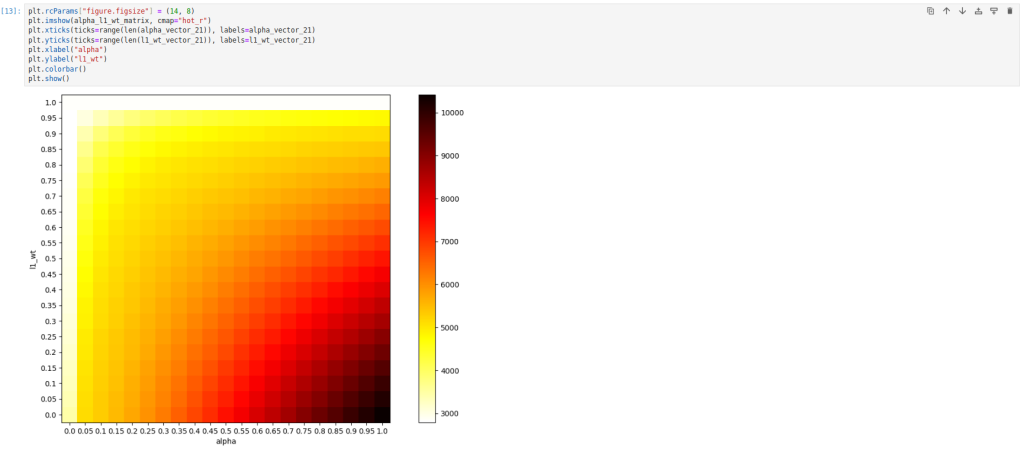

The lack of a proprietary implementation that makes use of cross-validation or supports parameters in vectors as in scikit-learn’s ElasticNetCV could lead to the conclusion that a Statsmodels implementation is more verbose or more limited. However, Statsmodels has an advantage over scikit-learn in the flexibility of handling penalties for cases where they wish to be applied in varying magnitudes on the different coefficients of the model. To do this, it is necessary to pass to the alpha parameter a vector of penalties of length equal to the number of variables.
A use case could be to apply penalties only to some coefficients of the model and not to all of them. For example, in the case of not wanting to impose any penalty to the variable “s1”, in position 5, the previous exercise could be repeated by imposing that alpha is 0 in position 5, iterating a constant value on the rest:


With the possibility of granting different penalties per variable, a range of additional dimensions opens up to eventually improve the predictive capacity of linear models. But, is it possible to establish some criterion with which to choose the weights per variable, without having to test the thousands of possible combinations? Regarding this issue, Tay et al. (2023) propose to modify the algorithms to assign a score to the variables based on a matrix where the “information about the predictors” (variables of variables) is represented in a method they call “feature-weight elastic net”, and whose implementation in Python does not exist at the date of publication of this entry (although they did program a package in R).
Conclusion
The application of L1 and L2 penalties are methods that can improve the predictive capacity in linear regressions, in addition to simplifying the models through an indirect selection of variables. Regularization by elastic netting allows both types of penalties to be applied simultaneously.
In Python, linear regressions with elastic net are implemented in the Statsmodels and scikit-learn packages. Scikit-learn has an implementation with cross-validation that is very easy to use, and Statsmodels, with the possibility of programming the cross-validation separately, offers interesting flexibility with respect to the handling of penalties at the variable level. However, exploiting all the possibilities that this flexibility can offer would require increasing the number of iterations by several magnitudes. As alternatives to the use of brute force, some algorithms have been proposed such as that of Tay et al. (2023) although as of today there is no implementation in Python.
Bibliography
– Hastie, T., Tibshirani, R., & Wainwright, M. (2015). Statistical learning with sparsity: the lasso and generalizations. CRC press.
– Tay, J. K., Aghaeepour, N., Hastie, T., & Tibshirani, R. (2023). Feature-weighted elastic net: using “features of features” for better prediction. Statistica Sinica, 33(1), 259-279. https://doi.org/10.5705/ss.202020.0226.
If you found this article interesting, we encourage you to visit the Data Science category to see other posts similar to this one and to share it on networks. See you soon!
