

In data science, forecasting is a widely used technique in data analysis. In this post, we’ll explore what NeuralProphet is and how it works—an open-source library designed to perform forecasting tasks.
What is forecasting?
In the fields of statistics and machine learning, forecasting is the process of making predictions about the future based on past and present data. Forecasts are widely used in decision-making, as they make it possible to define a strategy that aligns with the estimates produced by the models. Furthermore, they allow us to answer questions about the future in both the short and long term, depending on the model. For example, for weather models:
- Short term. To know whether to bring an umbrella, we can ask if it will rain in the next few hours.
- Medium term. When planning a trip, we can check what the weather is usually like in a specific month.
- Long term. To verify that climate change is occurring, we can ask whether temperatures will continue to rise over the years.
Forecasts are typically based on time series data collected at regular intervals (e.g., monthly, daily, hourly…) and predict a quantitative variable (e.g., number of sales, temperature…). For these time series, three patterns have been identified that the data may exhibit:
- Trend. This occurs when the data show long-term increases or decreases. It can be described as the direction in which the time series is moving.
- Seasonality. It happens when the data exhibit a pattern that repeats at fixed intervals within a year. These intervals are determined by the calendar. The most common seasonal patterns are annual (365 days), weekly (7 days), and daily (24 hours).
- Cycle. This occurs when the data reveals a pattern that repeats at irregular intervals. These cycles typically involve fluctuations spanning more than two years. For example, the rise or fall in sales depending on the economic situation.
What is NeuralProphet?
Time series forecasting is a broad and complex field. Just for the three points mentioned above, there are already many methodologies for fitting the data, each with its own hyperparameters to optimize. In addition, there are other factors—such as data autocorrelation (a value on one day may be linked to a previous day)—that add another layer of difficulty. For these reasons, people who are familiar with the data and should be the ones adjusting the models often do not have these models at their disposal.
Prophet is a library designed to simplify the forecasting process, making it accessible to more people and usable in many different frameworks. The model proposed by Prophet features default hyperparameter values that fit many time series and automatically evaluate the model.
The Prophet library was developed by Meta and released as open source in 2017. This library describes a time series in terms of three components: trend, seasonality, and holidays (or events). This type of decomposition is typical in forecasting models, as it allows the complexity of the time series to be broken down into independent parts with very clear meanings.
Drawbacks of Prophet
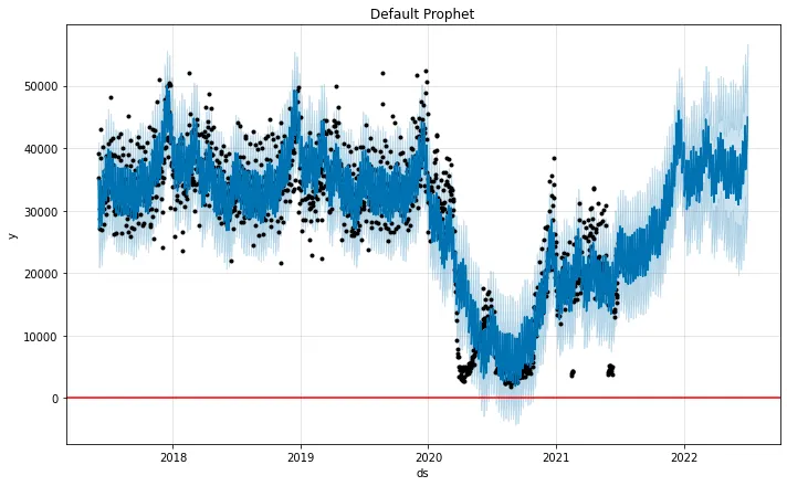
One of the main criticisms of Prophet is that the model is trained by fitting the best curve (as with linear regression) and does not learn the relationship between one time point and the next. In other cases, this is addressed, for example, with autoregressive (AR) models. This problem was clearly evident during the COVID-19 pandemic. Many time series experienced sharp drops and a change in behavior. While the model improved as it had more data in the new situation and was able to describe variations in the trend, the sudden change made forecasting for those dates unfeasible.
The following image shows an example from the official website for pedestrian traffic forecasting in Melbourne. Black represents the actual data, and blue represents the results of a Prophet model. The impact of COVID-19 is evident.
For these reasons, a new library, NeuralProphet, was released in 2021, adding three new components to those in Prophet: autoregression (past values of the variable to be predicted), backward regressors (other variables in the past), and forward regressors (other variables in the future). These three new components use a user-defined number of time points in the past or future. The first two are trained using neural networks.
Preprocessing and training with NeuralProphet
The library has some preprocessing steps configured by default. Specifically, it uses different techniques to impute missing values depending on the number of consecutive data points to be filled in. It also performs data normalisation, which can be customised by the user.
To ensure that the fitting is performed correctly, the time series is tabulated, and a pseudo-independent dataset is created. The model is trained using PyTorch and following stochastic gradient descent (SGD). Additionally, NeuralProphet has the following predefined components and hyperparameters, although they can be modified by the user:
- Loss function. The Huber function (smoothed L1) is used.
- Regularisation. The log of the absolute value of the weights is scaled and shifted.
- Optimiser. The AdamW optimizer is used.
- Learning rate. The optimal learning rate is determined by running three tests, and the results are averaged.
- Batch size. A value between 16 and 256 that depends linearly on the number of available points in the time series. If there are fewer than 16 points, all available points are used.
- Training epochs. A number between 50 and 500 that depends inversely on the number of points in the time series.
NeuralProphet components
The NeuralProphet model can be described as the sum of the components mentioned above:
ŷt
where, for a time step t:
- T(t) is the trend.
- S(t) is the seasonality.
- A(t) is the autoregressive effect.
- L(t) is the regression effect for variables with only a known past.
- F(t) is the regression effect for variables with a known future.
- E(t) is the effect of events and holidays.
These components can also be configured to combine multiplicatively rather than additively. The optimal configuration depends on the process being described.
NeuralProphet forecasts a number of future points at a time. This is a configurable parameter called the horizon (h). All components predict h points.
Sample dataset
In the following sections, we will examine some examples using air quality data from Spain and meteorological data from AEMET Open Data to attempt to predict the average daily NO₂ concentration in Palma. Data from the years 2017–2022 (both years included) have been used.
The hourly air quality data were filtered by province 7 (Balearic Islands), municipality 40 (Palma), and station 2 (avenidas) to obtain a single station, and by selecting parameter 8, which corresponds to NO₂. Next, an average was calculated across all hours of each day. This yields daily data on the average NO₂ concentration for a station in Palma. After reading the data, these are the transformations:
# Filter for traffic station in Palma (Avenidas)
df_air = df_air.loc[
    (df_air.PROVINCE == 7)
    & (df_air.MUNICIPALITY == 40)
    & (df_air.STATION == 2)
].copy()

# Get columns
df_air['ds'] = pd.to_datetime(df_air.apply(
    lambda s: f"{s['ANNO']:04d}-{s['MES']:02d}-{s['DIA']:02d}",
    axis=1
))
df_air['y'] = df_air[[f"H{h:02d}" for h in range(1, 25)]] \
    .mean(axis=1)
The meteorological data was retrieved from station B278 (Palma Airport). Daily metrics were obtained for average temperature (avgtemp), precipitation (prec), average wind speed (avgwind), average humidity (avghr), and hours of sunshine (sun). After reading the data, these are the transformations:
df_weather['ds'] = pd.to_datetime(df_weather['date'])

# Ip is <0,1
df_weather['prec'] = np.where(
    df_weather['prec'] == 'Ip',
    '0,1',
    df_weather['prec']
)

float_cols = ['avgtemp', 'prec', 'avgwind', 'avghr', 'sun']
for c in float_cols:
    df_weather[c] = df_weather[c].astype('str') \
        .str.replace(',', '.').astype('float')
Finally, the data from the two sources are combined:
# All dates
df = pd.date_range("2017-01-01", "2022-12-31") \
    .rename('ds').to_frame().reset_index(drop=True) \
    .merge(df_air, on='ds', how='left') \
    .merge(df_weather, on='ds', how='left')

cols = ['ds', 'y', 'avgtemp', 'avgwind', 'prec', 'avghr']
df = df[cols].sort_values('ds') \
    .reset_index(drop=True).copy()

DS_SPLIT_VALID = datetime(2022, 1, 1)
DS_SPLIT_TEST = datetime(2022, 7, 1)

df_train = df.loc[df.ds < DS_SPLIT_VALID]
df_valid = df.loc[
    (df.ds >= DS_SPLIT_VALID)
    & (df.ds < DS_SPLIT_TEST)
]
df_test = df.loc[df.ds >= DS_SPLIT_TEST]
Training, validation, and test dataframes are also created. Note that to use NeuralProphet, you need a dataframe from the Pandas library in Python that has two main columns: ds (the date as a datetime type) and y (the value to be predicted).
If you plot the resulting dataframe, you will see the following time series:
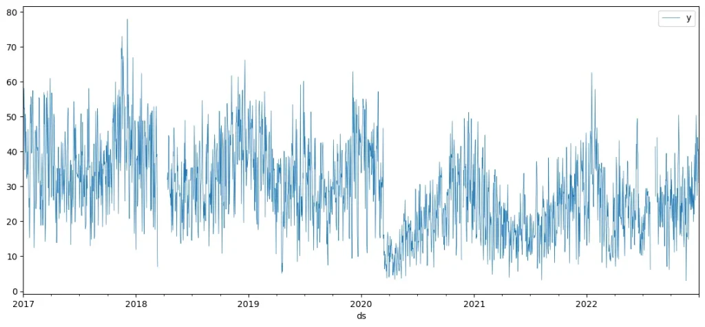
As we can see, there are two date ranges for which NO2 data is missing: around March 2018 and August 2022. The impact of the COVID-19 pandemic is also evident.
Trend
A classic way to model a trend is to use a straight line, where the slope represents the growth rate. NeuralProphet builds on this idea and introduces the concept of changepoints, which are points in time when the growth rate changes. Changepoints can be specified manually or automatically determined by the model. The result is a trend composed of several straight lines with different slopes connected at the changepoints.
In the following example, the NeuralProphet model has been trained using only the trend.
cols = ['ds', 'y']
m = NeuralProphet(
    weekly_seasonality=False,
    yearly_seasonality=False
)
m.fit(df_train[cols], validation_df=df_valid[cols])
Next, predictions are made for all the data, and these are plotted on a graph alongside the actual data to assess the fit:
forecast = m.predict(df[cols])
fig = m.plot(forecast, figsize=(14,8))

# ds split line
fig.add_vline(x=DS_SPLIT_VALID.timestamp()*1000,
              line_dash='dash',
              annotation_text='Validation')
fig.add_vline(x=DS_SPLIT_TEST.timestamp()*1000,
              line_dash='dash',
              annotation_text='Test')

# Prediction on top
fig.data = fig.data[::-1]
fig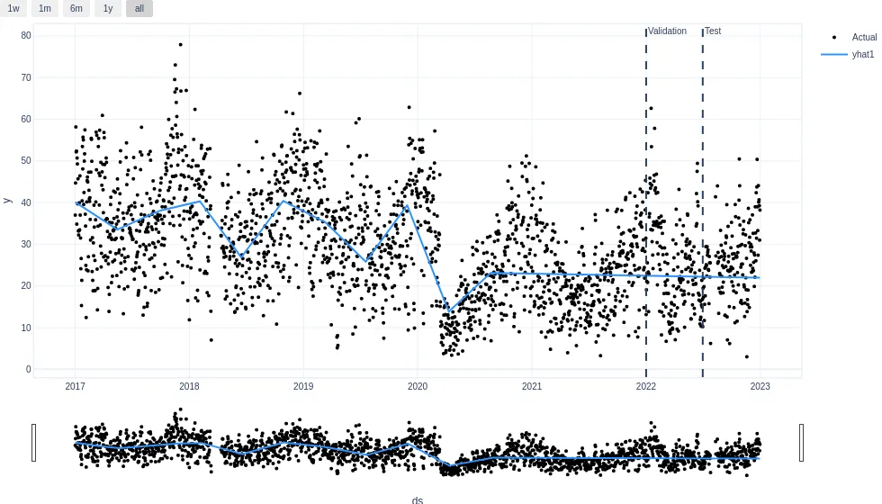
The graph shows that the forecast consists of a set of connected straight lines. The trend provides a general idea of the direction in which the time series is moving. Except for a trend reversal during the COVID-19 pandemic, it does not appear to vary much. By running plot_parameters, you can view the checkpoints and changes in the trend:
m.plot_parameters(figsize=(14,4))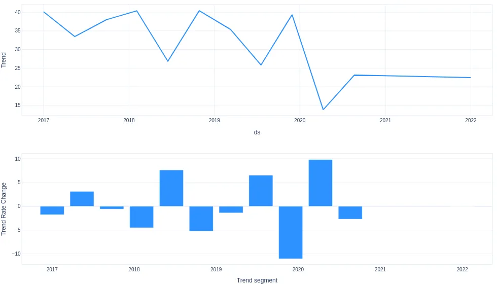
Seasonality
The seasonality component in NeuralProphet is defined as a k-term Fourier series. You can configure more than one periodicity (p) at a time, fitting a Fourier series for each one. The total effect of seasonality is the sum of all of them.
If nothing is configured, the model analyzes the data’s time scale (monthly, daily, hourly, etc.) and checks for periodicity across possible periods, focusing on those smaller than the time scale and with sufficient data. Additionally, for each period, the model determines a number of Fourier terms (k) that works well. Alternatively, you can configure these two parts manually.
Next, take the previous model and enable automatic seasonality. The model in this example is equivalent to instantiating NeuralProphet without any parameters, since by default it fits a trend and the possible seasonal components.
cols = ['ds', 'y']
m = NeuralProphet()
m.fit(df_train[cols], validation_df=df_valid[cols])
Once again, the graph showing the model fit is displayed. The model looks similar to the previous one, but now the lines are oscillating curves that attempt to better match the variations in the data.
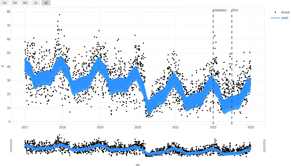
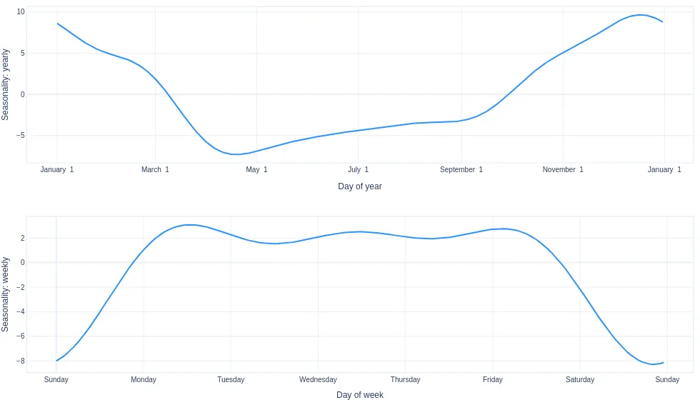
Weekly seasonality is barely noticeable at this scale. However, it is possible to see how the fluctuations recur at the same time of year. For example, just before the end of the year, there appears to be a peak in this seasonality. This could coincide with the Christmas season. To get a better view of each component, the parameter plot is shown again:
Autoregression
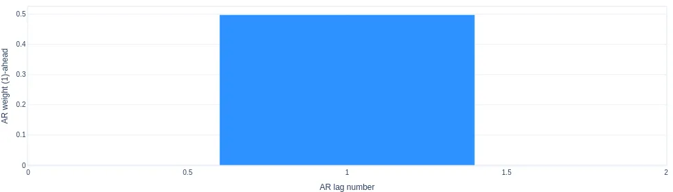
The autoregression component attempts to describe the dependent variable (yt) based on its past values (yt-1, yt-2, etc.). NeuralProphet relies on the AR-Net model to evaluate this component. This model uses neural networks in PyTorch to identify complex relationships among past values that enable a prediction. The neural network has a number of inputs equal to the number of past data points to be used and a number of outputs equal to the horizon (h).
cols = ['ds', 'y']
m = NeuralProphet(n_lags=1)
m.fit(df_train[cols], validation_df=df_valid[cols])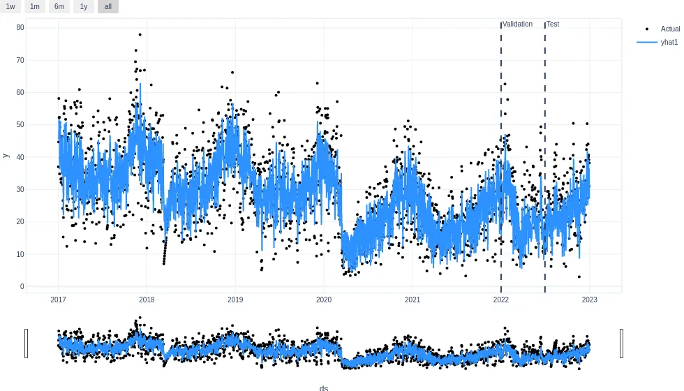
Next, the parameters are displayed again. Here, the command is modified slightly to ensure that, if there is more than one lag, the first one is displayed:
m.plot_parameters(
    figsize=(14,4),
    components=['autoregression'],
    forecast_in_focus=1
)
Past regressors
The regression component for past variables attempts to describe the dependent variable (yt) as a function of past values of other independent variables (xt-1, xt-2, etc.). Each of these variables is estimated using AR-Net again. The only difference from the autoregression component is the input variable to the neural network.
One hypothesis might be that wind is capable of moving NO₂, thereby influencing its concentration. Next, the new regressor avgwind is added to the previous model, and a single lag is configured, just as in the autoregressive component.
cols = ['ds', 'y', 'avgwind']
m = NeuralProphet(n_lags=1)
m.add_lagged_regressor("avgwind", n_lags=1)
m.fit(df_train[cols], validation_df=df_valid[cols])
The results and parameters are shown below:
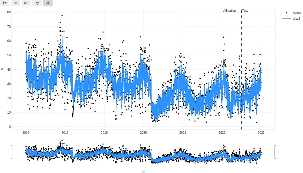
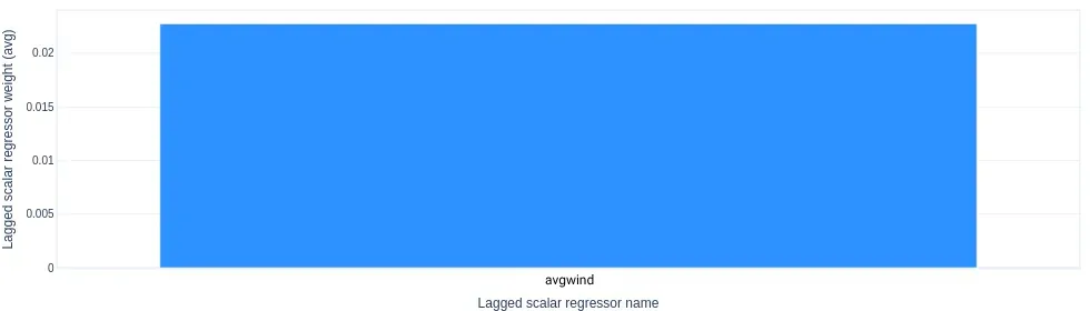
As can be seen, this variable has a relatively small weight compared to the autoregressive component.
Forward regressors
The regression component for variables with a known future value attempts to describe the dependent variable (yt) in terms of the past and future values of independent variables. These variables must be predicted by other models or known in advance at the time of predicting yt.
In this example, average temperature data is added. Since this is a forward regressor, it is assumed that an external system for forecasting the average temperature is available.
cols = ['ds', 'y', 'avgwind', 'avgtemp']
m = NeuralProphet(n_lags=1)
m_future_regressors.add_lagged_regressor("avgwind", n_lags=1)
m_future_regressors.add_future_regressor("avgtemp")
m.fit(df_train[cols], validation_df=df_valid[cols])
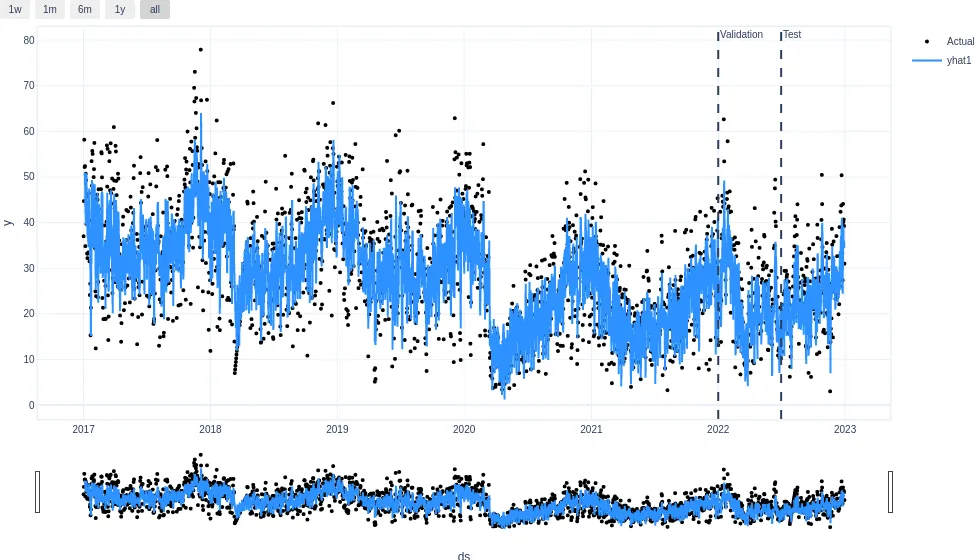
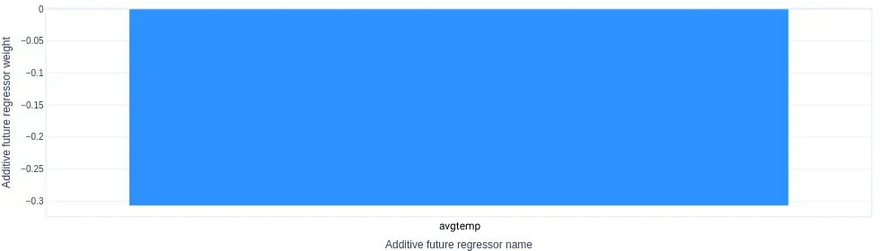
The model is trained, and the following graphs are obtained:
Events
The events and holidays component aims to describe the impact that certain dates have on the dependent variable (yt). For country-specific holidays, NeuralProphet integrates the python-holidays library, so that you only need to specify the desired country. Users can also define custom events—such as concerts, soccer games, or extreme weather—by specifying the dates on which they occur. It is also possible to define a time window around these events to indicate that adjacent days may be affected.
For this use case, Spanish holidays are added:
cols = ['ds', 'y', 'avgwind', 'avgtemp']
m = NeuralProphet(n_lags=1)
m_future_regressors.add_lagged_regressor("avgwind", n_lags=1)
m_future_regressors.add_future_regressor("avgtemp")
m.add_country_holidays('ES')
m.fit(df_train[cols], validation_df=df_valid[cols])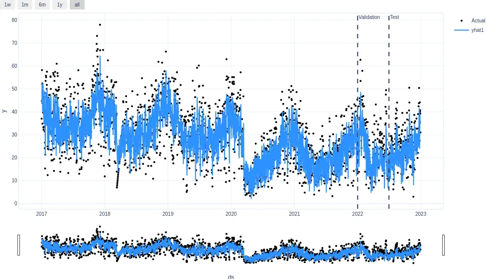
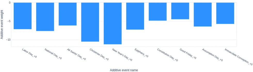
A negative effect of all holidays on NO2 concentrations can be observed.
Comparison
In the previous examples, components were added incrementally, and the results were evaluated visually. Next, the model is expanded in two ways:
- First, the number of autoregressive lags and the number of past variables are increased from 1 to 3.
- Second, the past variables hrMedia and prec are added.
The resulting code is as follows:
cols = ['ds', 'y', 'avgtemp', 'avgwind', 'prec', 'avghr']
m = NeuralProphet(n_lags=3)
m.add_lagged_regressor("avgwind", n_lags=3)
m.add_lagged_regressor("avghr", n_lags=3)
m.add_lagged_regressor("prec", n_lags=3)
m.add_future_regressor("avgtemp")
m.add_country_holidays("ES")
m.fit(df_train[cols], validation_df=df_valid[cols])
Finally, to obtain a numerical result, the test method is used to evaluate a series of metrics. The RMSE is selected and compared with the previous models:
| T(t) | S(t) | AR(P)(t) | L(P)(t) | F(t) | E(t) | RMSE |
| linear | – | – | – | – | – | 9.47 |
| linear | yearly weekly | – | – | – | – | 8.86 |
| linear | yearly weekly | AR(1) | – | – | – | 7.13 |
| linear | yearly weekly | AR(1) | avgwind(1) | – | – | 7.10 |
| linear | yearly weekly | AR(1) | avgwind(1) | avgtemp | – | 7.17 |
| linear | yearly weekly | AR(1) | avgwind(1) | avgtemp | ES | 7.01 |
| linear | yearly weekly | AR(3) | avgwind(3) avghr(3) prec(3) | avgtemp | ES | 6.84 |
Conclusion
NeuralProphet is a forecasting library designed to be simple. Throughout this post, we have seen how, with minimal configuration, we can obtain decent results because the library automatically adjusts various parameters behind the scenes. The separation into different components allows us to model various typical behaviors of time series.
If you found this article interesting, we encourage you to visit the Data Science category to see other posts similar to this one and to share it on social networks. See you soon!
