Simple Perceptron: Python implementation

Introduction

Artificial neural networks are one of the main lines of study in the field of artificial intelligence today. This family of algorithms allows solving tasks as complex and diverse as image recognition, natural language processing or music generation. The main constituent unit of these models is the simple perceptron, which essentially mimics the basic functioning of a biological neuron.

As we explained in the last post Simple Perceptron: Mathematical Definition and Properties, its operation can be summarized as follows.

We start with a set of input data, each with a number of independent or explanatory variables x⃗ = (x₁,… ,x_N) and a dependent or target variable y. The purpose of the perceptron is to learn how to predict the variable y from the variables x⃗, and to do so it needs to learn from a dataset called the training set. Thus, given an observation (x⃗⁽ⁱ⁾, 𝑦⁽ⁱ⁾), the model outputs a prediction ŷ⁽ⁱ⁾ according to the function

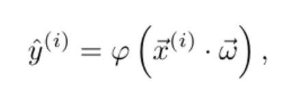
where φ is the activation function and ω⃗ = (ω₁,…,ω_N) is the vector of weights, which is initialized randomly.

How does the model learn? After each input example, the predicted value is compared with the actual value, in order to quantify the error made by means of a cost function (or loss function) 𝐽(x⃗⁽ⁱ⁾, 𝑦⁽ⁱ⁾). Note that, given an input vector x⃗⁽ⁱ⁾, the predicted value depends only on the weights, so given a training example (x⃗⁽ⁱ⁾, 𝑦⁽ⁱ⁾), the cost function depends only on the vector of weights, 𝐽 = 𝐽(ω⃗).

Thus, knowing the gradient of the cost function with respect to the weights ∇𝐽(ω⃗), we can use gradient descent to update the weights as we make predictions and thus minimize the cost function. As we saw, there are different variants of gradient descent, depending on the frequency with which the weights are updated: stochastic gradient descent, in which the weights are updated after each training example; minibatch gradient descent, in which they are updated after a certain number of examples; and batch gradient descent, in which the update occurs after each epoch, or loop over the entire training set.So, the update of the weights ω⃗^(𝑘) at each iteration 𝑘 is given by the formula

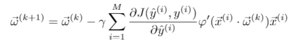
where 𝛄 is the learning rate and the summation runs through a number 𝑀 of training examples, which depends on the gradient descent mode used. Note that the chain rule has been used to calculate the gradient of the cost function with respect to the vector of weights, ∇𝐽(ω⃗^(𝑘)), as a function of the predicted value ŷ⁽ⁱ⁾ = ŷ⁽ⁱ⁾(ω⃗^(𝑘)).

Example of implementation in Python

To better illustrate the whole process described above, let’s look at a specific example.

Suppose that we work in a bank and we want to build a model that predicts whether a customer will repay a loan or not, based on only two independent variables: the amount of the loan granted and the customer’s monthly income. To do this, we need a training set consisting of many observations of customers for whom we know these two variables, as well as whether they repaid the loan or not.

import pandas as pd
data = pd.read_csv("loan_data.csv")

data.head()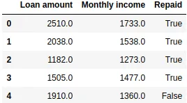

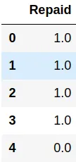
We have a pandas.DataFrame in which the first two columns represent, respectively, the loan amount and the customer’s monthly income (expressed in certain monetary units) and the third column contains the dependent variable: True if the loan was repaid and False otherwise.

It is common that the different variables in our dataset have different orders of magnitude. Therefore, it is usual to first perform a normalization of the data: in this case, we linearly scale each of the numerical variables in the interval [0, 1].

from sklearn.preprocessing import MinMaxScaler

indep_vars = ["Loan amount", "Monthly income"]
data[indep_vars] =  MinMaxScaler().fit_transform(data[indep_vars])
data.head()

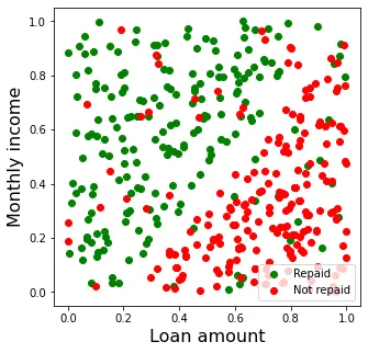
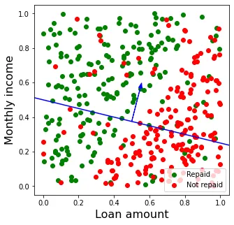
Figure 1 shows a scatter plot of the data available to us. In general, there is a pattern in the data: the loan is repaid in most cases where the loan amount is low in relation to the client’s monthly income (upper left part of the graph), while it is not repaid in cases where the loan amount is relatively high (lower right part).

In this case, since we have a binary variable, we will use the logistic activation function, whose expression and that of its derivative are given by

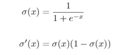
Because this function always gives an output between 0 and 1, in the case of binary classification it can be interpreted as the probability ŷ = 𝑃 (𝑦 = 1). Furthermore, the function is increasing, and it is fulfilled that σ(0) = 0.5. So, given the linear combination between weights and independent variables, 𝑧 = x⃗ · ω⃗, we will have that σ(𝑧) = ŷ > 0.5 (and therefore the prediction will be 𝑦 = 1) if and only if it is satisfied that 𝑧 > 0. This means that the vector of weights determines a hyperplane (in our two-dimensional case, a straight line) that divides the plane into two regions, such that for all points in one region we have ŷ > 0.5 (in our case, we predict that the loan will be repaid) and for all points in the other region we have ŷ < 0.5 (we predict that the loan will not be repaid).

Note that, if we only considered as many weights as independent variables (two in our case: ω₁ and ω₂), we would have the line

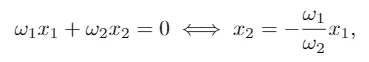
which always contains the origin of coordinates. In order to fit the Y-intercept of the line determined by the vector of weights (or in the case of 𝑁 explanatory variables, the independent term of the hyperplane that divides the space into two regions), an additional variable 𝑋₀ consisting of a column of ones is usually introduced as an input to the model. In this way, its associated weight ω₀ will adjust the independent term of the hyperplane.

Thus, we separate our dataset into the independent variables X and the target variable y, which we convert to numerical: (False, True)→(0,1). We also introduce the additional variable X0 as a column of ones

X = data[indep_vars]
y = data[["Repaid"]].astype(float)
X.insert(0, "X0", 1.)

X.head()
y.head()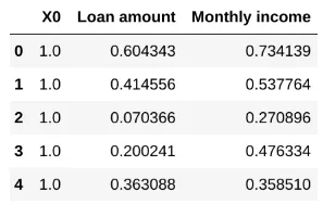

We next divide the dataset into the training, validation and test sets.

from sklearn.model_selection import train_test_split

X_train, X_test, y_train, y_test = train_test_split(X.values, y.values, test_size=0.3)
X_train, X_validation, y_train, y_validation = train_test_split(X_train, y_train, test_size=0.3)

We are now ready to define our simple perceptron. Of course, there are libraries such as scikit-learn or keras that contain neural network implementations, including the simple perceptron case. For example, using the SGDRegressor or  SGDClassifier classes of the  sklearn.linear_model module, we can instantiate a perceptron that uses stochastic gradient descent (SGD) depending on whether we are dealing with a regression or a classification problem, respectively. 

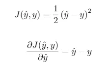
However, to better illustrate the concepts, we will now define our own class, which we will call SimplePerceptron. In this case, we will use the quadratic loss function. As we saw in the aforementioned post Simple perceptron: Mathematical definition and properties, its expression and that of its derivative are given by

Another common choice in the case of binary classification is the binary cross entropy, given by the equation

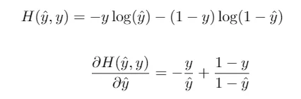
In fact, by combining this loss function with the logistic activation function, we obtain the popular logistic regression algorithm.

Finally, we use the batch gradient descent and set a fixed learning ratio of 𝛾 = 0.1 during training.

class SimplePerceptron:
    learn_rate = 0.1

    def __init__(self):
        self.weights = None
        
    def logistic_function(self, x: float) -> float:
        """
        Logistic function, used as the activation function
        """
        return 1. / (1 + np.exp(-x))

    def forward_pass(self, X: np.ndarray) -> float:
        """
        Prediction of a single data point, given the current weights
        """
        weighted_sum = np.dot(X, self.weights)
        output = self.sigmoid_function(weighted_sum)

        return output

    def fit(self, X_train: np.ndarray, y_train: np.ndarray, n_epochs: int = 20):
        """
        Training using Batch Gradient Descent.
        Weights array is updated after each epoch
        """
        self.weights = np.random.uniform(-1, 1, X_train.shape[1])
        current_weights = self.weights.copy()
        for epoch in range(n_epochs):
            for x, y in zip(X_train, y_train):
                y_predicted = self.forward_pass(x)
                current_weights -= self.learn_rate * (y_predicted - y) * y_predicted * (1 - y_predicted) * x
            self.weights = current_weights.copy()

    def predict(self, X_test: np.ndarray) -> np.ndarray:
        """
        Predict label for unseen data
        """
        return np.array([self.forward_pass(x) for x in X_test])

From here, we can train the model by passing the training data to the fit() function, and once trained, we can use the predict() method to make predictions on the test data.

perceptron = SimplePerceptron()

perceptron.fit(X_train, y_train)
y_pred = perceptron.predict(X_test)

To see how the learning process unfolds step by step, we will illustrate it with the results of a single execution of the above command. First, the vector of weights is randomly initialized, and we obtain a value ω⃗⁽¹⁾ = (-0.39, 0.21, 0.80). This vector divides the plane into two regions, as shown in Figure 3.

With this division, all points above the line are predicted as green (𝑦 = 1 or loan repaid) and all points below are predicted as red (𝑦 = 0 or loan not repaid).  Obviously, since this is a random initialization of the vector of weights, the error committed is high: in particular, all points in red above the line and all points in green below it will be incorrectly classified. This yields an accuracy score (number of correctly classified examples  divided by total number of examples) of 0.575 on the test set. Since a random binary classification has an expected precision score of 0.5, we confirm that the initial classification is rather poor.

Then the training process starts: in each epoch, all the training examples are run through, calculating their prediction (Equation 1) using the current vector of weights. Note that the corrections in the weights (Equation 2) are stored in the current_weights variable after each prediction. However, since we use batch gradient descent, the variable self.weights (the one used to make the predictions in the forward_pass() method) is only updated at the completion of each epoch.

At the end of the first epoch, the loss function over the total dataset is 𝐽(ω⃗⁽¹⁾) = 46.37. After applying the first update of the weights, we obtain a new vector of weights ω⃗⁽²⁾ =(-0.46, -0.18,  0.98), calculated by accumulating the corrections corresponding to each prediction. Thus, in the second epoch we obtain a cost function 𝐽(ω⃗⁽²⁾) = 44.70 which is lower than 𝐽(ω⃗⁽¹⁾), reflecting that we moved in the decreasing direction of the function. 

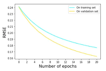
The same procedure is repeated for each of the subsequent epochs, obtaining a decreasing value of the cost function. Figure 4 shows the evolution of the RMSE metric (proportional to the square root of the loss function) on the training and validation sets after 20 epochs. In this case we see that the loss function shows a decreasing trend for both the training and validation sets, which indicates that no overfitting has occurred. In fact, except for a very biased choice of training data, it is difficult for a model as simple as the perceptron to overfit the data.

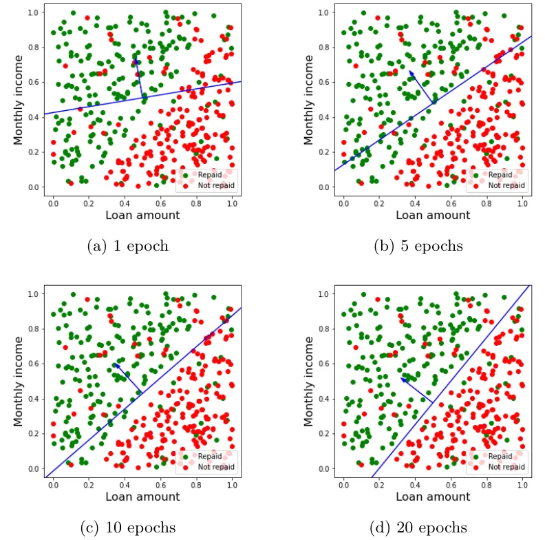
Finally, Figure 5 shows the evolution of the division of the plane by the vector of weights after different numbers of epochs. As we can see, although a perfect classification is not achieved, at the end of the training process the line determined by the weights is able to separate the two classes much better than with the initial vector of weights, as a result of the corrections introduced at the end of each epoch.

After this process, the accuracy score of the model on the training set is 0.90, well above the initial score of 0.575.  The accuracy score on the test set is 0.8875, very close to that obtained for the training set, again a sign that the training data have not been overfitted. This means that, knowing the client’s income and the loan amount, we will correctly predict whether the loan will be repaid or not in about 9 out of 10 cases.

Note that, given our dataset, we can never achieve an accuracy score of 1.0 (which would mean no classification error) with this model. This is because the data are not linearly separable, i.e., you cannot perfectly separate the green and red dots using a straight line. In fact, this is one of the fundamental limitations of the simple perceptron: being a linear model (using linear combinations of the input variables, like for example logistic regression does) it is only able to perfectly learn datasets which are linearly separable in the explanatory variables.

Next Steps

In future posts we will discuss how simple perceptrons can be combined to build artificial neural networks, and how these can help solve more complex problems, in particular those where data are not linearly separable. In the meantime, we encourage you to visit Damavis‘ blog and see articles similar to this one in the Algorithms category.

If you found this post useful, share it with your contacts so that they can also read it and give their opinion. See you in social networks!