One of the most common problems in data science is predicting the value of certain variables based on others. For example, we need to know whether it is advisable to grant a loan to a customer depending on factors such as their age, monthly income, etc. To do this, we simply need to classify each case into two categories: whether we grant the loan or not. Therefore, we are faced with a classification problem.
Another example would be estimating the price of a house based on its characteristics (age, surface area, number of rooms, location, etc.). In this case, we want to predict a quantity (the price of the house). This is considered a regression problem.
Classification and regression problems are the two main classes of what is called supervised machine learning. In this paradigm, a mathematical model is trained to learn to predict one or more variables (dependent or target variables), from others (independent variables).
Predictions and relationships between variables
In order to understand how the different variables are related to each other and to be able to make a prediction, we need to start from a set of observations. In the example of estimating house prices, we should have many examples of homes for which we know both the independent variables (age, surface area, and other characteristics) and the dependent variable (price). During the training process, the model must understand how the different characteristics of the house affect its price. This way, it will later be able to predict the price of a house based solely on the other variables.
There are many different supervised learning models that can be used to tackle both classification and regression problems. Among the most popular algorithms are K-Nearest Neighbors (mostly used for classification), logistic regression (or classification and regression) or linear regression (for regression).
However, most of these algorithms have limitations for solving problems where the data structure is relatively complex. Thus, for example, logistic regression fails for classification problems where the data are not linearly separable.
To solve complex problems, a set of models with a common structure has been developed and popularized in recent decades. These are known as artificial neural networks.
Artificial neural networks
Let’s start with the basics: what are neurons? They are the cells responsible for the propagation of nerve impulses through the nervous system of animals.
These cells consist of two main parts. On one hand, there is the cell body or soma, from which short extensions called dendrites protrude. On the other hand, there is a long extension called the axon, which connects to other neurons. The dendrites are responsible for transmitting the impulses they receive from other cells to the soma. From there, the impulse spreads through the axon. Finally, they are transmitted to another neuron via the neuronal synapse (or to a motor cell).
Neural networks are thus made up of trillions of neurons connected to each other. It is this architecture that enables animals to learn.
Artificial neural networks aim to mimic the functioning of biological neural networks. In the same way that biological neural networks are composed of neurons, the main constituent unit of artificial neural networks is the simple perceptron. The perceptron is nothing more than the mathematical representation of a neuron. In fact, it mimics its structure and the functions of each of its parts. Not surprisingly, it is often referred to as an artificial neuron. Let’s take a look.
The simple perceptron
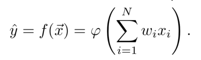
A perceptron can be defined as a mathematical function f that allows relating a vector of independent variables x⃗ = (x1,… ,xN) , with a dependent variable y , so that the independent variable is estimated as ŷ = f(x⃗) . This function is parameterised by a vector of weights, ω? = (ω1,…,ωN)T , which weight the influence of each of the independent variables on the value of the dependent variable, and by a function φ, called the activation function, such that
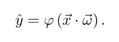
In fact, the linear combination can be expressed as a scalar product between the vector of independent variables and the vector of weights. In this way, the above equation can be expressed as
Biological neuron and artificial neuron
So far, you may not see the perceptron’s resemblance to a neuron. But how about painting it like this
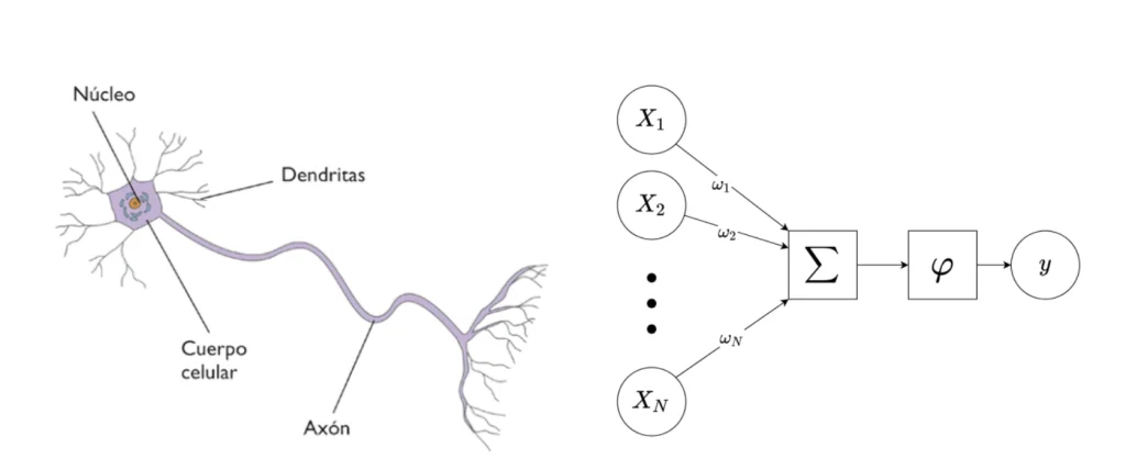
Let us study from Figure 1 the analogy between a biological neuron and an artificial neuron. Each of the input variables (here the x1,… ,xN) represents the signal received by the neuron through the synapse with a neighbouring neuron. All these inputs are combined with each other through a simple operation. Each input value xi is multiplied by a weight ωi. This weight weights the contribution of that variable in the calculation of the dependent variable. All these contributions are then added together.
This operation simulates the transmission and combination of all input signals through the dendrites to the centre of the neuron. Finally, the effect of the activation function φ on the weighted sum represents how information propagates through the axon.
Activation function and step function
The activation function transforms the result of the linear combination between the independent variables and their associated weights. As its name suggests, its purpose is to determine the activation level of the neuron. The simplest activation function is called the step function, defined as
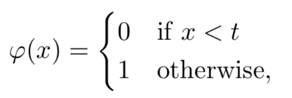
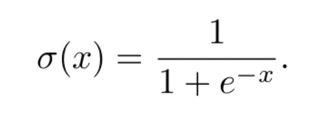
where t is a parameter of the model. With this example, the neuron’s output will be 1 (we say that the neuron will be activated, or that its information will propagate through the axon) if and only if the linear combination exceeds the threshold value t. Otherwise, its result will be 0. Although this function is very intuitive, it has the disadvantage of not being derivable. In the learning process, we need the functions involved to be derivable. For this reason, other activation functions are used. One of the most commonly used is the logistic function, defined by the formula
This function is indeed differentiable, and in fact its derivative satisfies the simple equation
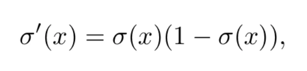
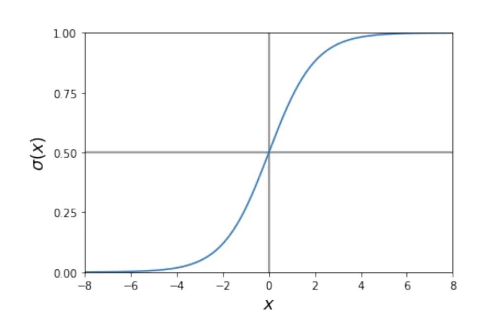
which greatly simplifies the learning process. The shape of the logistic function can be seen in Figure 2. For arbitrarily positive values of x, it tends to one. In the case of arbitrarily negative values, it tends to 0, satisfying σ(0) = 0.5. Thus, the neuron will activate (ŷ = 1) if the linear combination is very positive. Conversely, it will turn off (ŷ = 0) if it is very negative.
Perceptron learning
Now, what does the perceptron learning process consist of? Well, it is about finding the weights ωi that best fit the data we have.
This data consists of a (preferably large) set of observations in which we know both the independent variables and the variable we want to learn to predict. The idea is that, for each input example, the model tries to predict the target variable from the independent variables. At first, it will make many mistakes. However, since we know the actual value of the variable to be predicted, it will correct itself after each prediction so that it will give better results each time.
The first step in any supervised learning algorithm is to divide the dataset into two parts. A training set and a test set. The training set, as its name suggests, is used to build the model, while the test set serves to validate it once the training process is complete.
The loss function
In order to assess how good a prediction is in order to give feedback to the model during the training process, we must define a loss function. This function J(ŷ, y) should quantify the error made in estimating the value of y in each prediction ŷ.
In regression problems, where the dependent variable is continuous, the simplest choice would be to take the absolute value of the difference between the actual and predicted value. This is, J(ŷ, y) = |ŷ – y|. However, once again, we find that this function does not satisfy the desired property of derivability. Therefore, other loss functions are preferred.
One of the simplest (and also one of the most widely used) is the quadratic difference, defined by equation
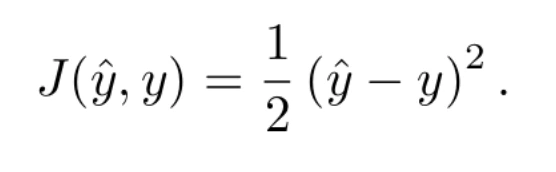
This equation has the advantage that it is differentiable. In fact, its derivative can be expressed as
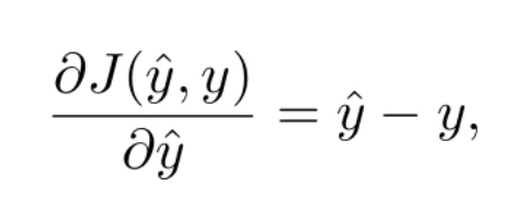
which is nothing more than the error (with sign) made in the prediction.
The gradient descent
Why so much stress on functions being differentiable? The reason is that to find the value of the weights that solve the problem, the neural network relies on an iterative method, gradient descent.
How it works
This method, in general, aims to find the minimum of a certain function F by calculating its gradient. That is, the derivative with respect to its input parameters x⃗. The method works as follows:
- The input parameters, x⃗(1), are either first estimated or randomly initialised.
- For each iteration k =1, 2, …
- The gradient of the function with respect to the current parameters is calculated

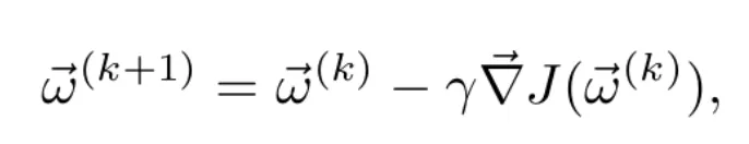
- Since the gradient points in the direction of maximum growth of the function, and the objective is to minimize the function, the parameters are updated by introducing a small variation in the opposite direction to that of the gradient. The rule to be applied is
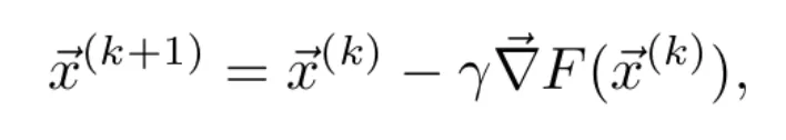

where is a real number that determines how much the parameters are modified in each iteration. For values of 𝛄 small enough, it is satisfied that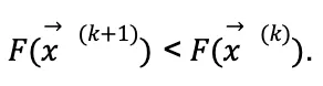
 . That is, for each iteration the value of the function will be reduced.
- The gradient of the function with respect to the current parameters is calculated
- Stopping criterion: we can set a maximum number of iterations, or a minimum threshold in the variation of the parameters. The idea behind the second method is to stop when gradients close to zero are obtained. In the case where F is a convex function, this indicates that we are close to the absolute minimum.
Gradient descent and perceptron
In the case of the perceptron, our goal is to find the vector of weights ω⃗ that minimizes the loss function. To do this, we need to be able to calculate the gradient of the loss function with respect to the weights based on the training result. Therefore, we need all the functions involved in the process to be differentiable. Thus, whether it is ![]()
![]() be the weight vector in iteration k, the update rule (Equation 8) is
be the weight vector in iteration k, the update rule (Equation 8) is
where the learning rate 𝛄 can be fixed as a hyperparameter of the model or adjusted as training progresses. A common technique, especially in the case of convex loss functions with respect to the weights, is to use a fading learning rate throughout the training. In this way, as we approach the minimum, the variations in weights are smaller. This prevents us from leaving the minimum’s basin of attraction or oscillating indefinitely around it (see Figure 3).

Variations in gradient descent
In general, the gradient descent method in neural networks consists of running through the entire training set (usually several times), where each loop over all examples is called an epoch. The weights are updated throughout the workout. Depending on when and how this update is applied, we have different variants of the gradient descent. We summarize them below.
Batch gradient descent
In this gradient descent method, the weights are updated after completing each epoch. That is, each time the entire training set has been run through. In this way, the contribution of all training examples to the gradient of the loss function is taken into account. In addition, the weights are updated in such a way as to minimize the error across the entire dataset.
This technique yields very good results when the loss functions are convex or relatively smooth. This is because it converges directly to the minimum (local or absolute). However, it has a major disadvantage. For relatively large data sets (as is often the case), it is computationally very expensive.
Stochastic gradient descent
In this variant, weights are updated with each training example. Once an epoch has been completed, it is common practice to randomly reorder the training set before restarting the loop. This prevents a fixed order from affecting the result.
This technique has the advantage that it is computationally much lighter than the previous one. However, as its name suggests, the evolution of the cost function becomes stochastic. In each iteration, the value of the cost function is reduced for the example in question.
However, the overall cost function may worsen. This property may be desirable when the loss function is not convex, as it allows us to escape from the basin of attraction of a local minimum toward another, better local minimum. However, it does not ensure convergence to the minimum, as it tends to oscillate due to its stochastic nature.
Gradient descent in minibatch
This variant combines the best of the previous two. Instead of using a single training example or all of them, a subset of training examples is used. This subset, known as a minibatch, is used to update the weights in each iteration until the entire dataset has been covered after n=M/k iterations. (Where M is the number of training examples and k is the size of the minibatch).
As in the previous example, once all the examples have been processed, they are usually reordered to ensure randomness. In this way, by having a sample that is more representative of the total than a single example, the average contribution of the minibatch usually causes the total cost function to tend to decrease with each iteration.
However, randomness leaves room for a possible escape from a suboptimal local minimum to a better minimum. The size of the minibatch k is a hyperparameter of the model. The ideal balance is for it to be small enough to escape suboptimal minima, but large enough to converge if it is close to the global minimum, which usually has wider and deeper basins of attraction.
We have already chosen the descent mode based on the characteristics of our problem. All that remains is to calculate the gradient of the loss function with respect to the weights that appear in Equation 9.
Calculating the gradient of the loss function
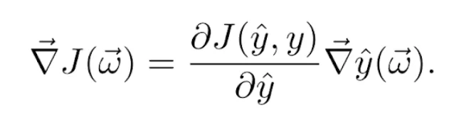
Let us assume for the moment that we use the stochastic gradient descent, and we will see later how it generalizes to the other variants. Let (x⃗, y) be the training example in question, and let ŷ be the prediction obtained using the current weight vector ω⃗. We know that the cost function J(ŷ, y) depends on the predicted value ŷ, which in turn depends on ω⃗, so to calculate its gradient with respect to the weights, we use the chain rule:
The gradient of the predicted value with respect to the weights is calculated by again using the chain rule on Equation 2, so that
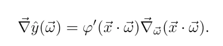
The gradient of the scalar product with respect to the vector of weights is x⃗. Finally, putting Equations 9, 10 and 11 together, the weights’ update rule becomes
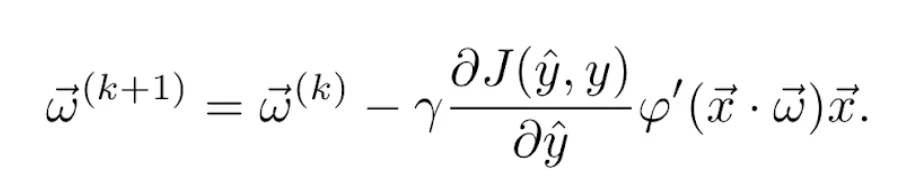
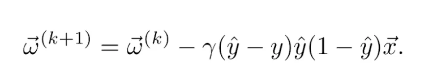
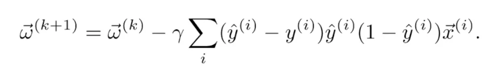
For example, let us consider the logistic activation function defined in Equation 4 and the quadratic loss function defined in Equation 6. Their derivatives are given, respectively, by Equations 5 and 7, so the update rule becomes
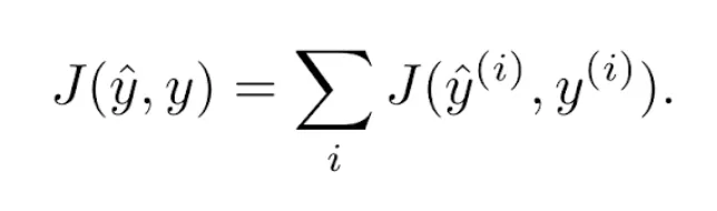
In the case of batch or minibatch gradient descent, the loss function is usually considered as the sum of the errors made in the predictions ŷ(i) of all training examples (x⃗(i), y(i)) considered in each iteration (being, in the case of batch gradient descent, the total number of examples M, and in the case of minibatch gradient descent, the minibatch size k):
The derivative of the sum is equal to the sum of the derivatives, so the rule for updating the weights becomes
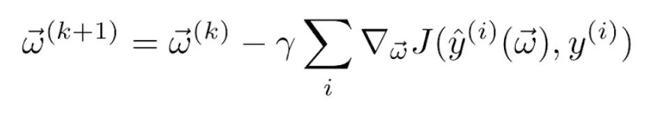
for each epoch k. In the case of using the quadratic loss function and the logistic activation function as in the previous example, we again get the weights’ update rule
Number of epochs and overfitting
Finally, let’s talk about how to determine another hyperparameter of any neural network, which is the number of epochs to be performed. In fact, this number is usually not fixed, but rather a stopping rule.
The idea is that the model must be able to learn the general structure of the training data in order to make good predictions, but overfitting must be avoided, that is, learning the particular characteristics of this data (such as noise). In this way, the model is intended to be generalizable to unseen data examples.
Typically, too low a number of epochs will not be sufficient for the model to fit the training data, while too large a number is likely to overfit the data, while of course increasing training time.
Model training
To determine when to stop training, the following procedure is commonly used. When we divide the dataset into training and test, we further subdivide the training set and keep a part of it as a validation set. In this way, the model is trained only with the rest of the training set, and we study how the loss function (or other metrics) evolves on both this set and the validation set throughout the training process, usually after each update of the weights.
As the model is trained with the objective of minimising the cost function on the training set, we will generally observe that the result of the model on this set always improves. However, it is common that after some epochs the result starts to worsen over the validation set: at this point overfitting is happening, and we must end the training process (this is called early stopping). As long as overfitting does not occur, we can continue training until we reach a target accuracy level or a predetermined maximum number of epochs.
In fact, in the case of the simple perceptron the model is very simple and is not able to learn very specific features of the data. Thus, overfitting is rare, being more common in more complex neural networks, as we will see in the following posts.
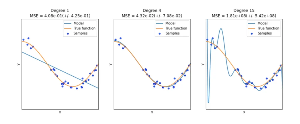
Underfitting and overfitting in polynomial regression
A canonical case is that of polynomial regression: if we choose too low a degree, the model will not be complex enough to understand the distribution of the data (this is also called underfitting), while if the degree is too high, the model will learn the specific features of the training set, including noise, and will not be generalizable. Figure 4 shows an example of underfitting and overfitting in the case of polynomial regression.
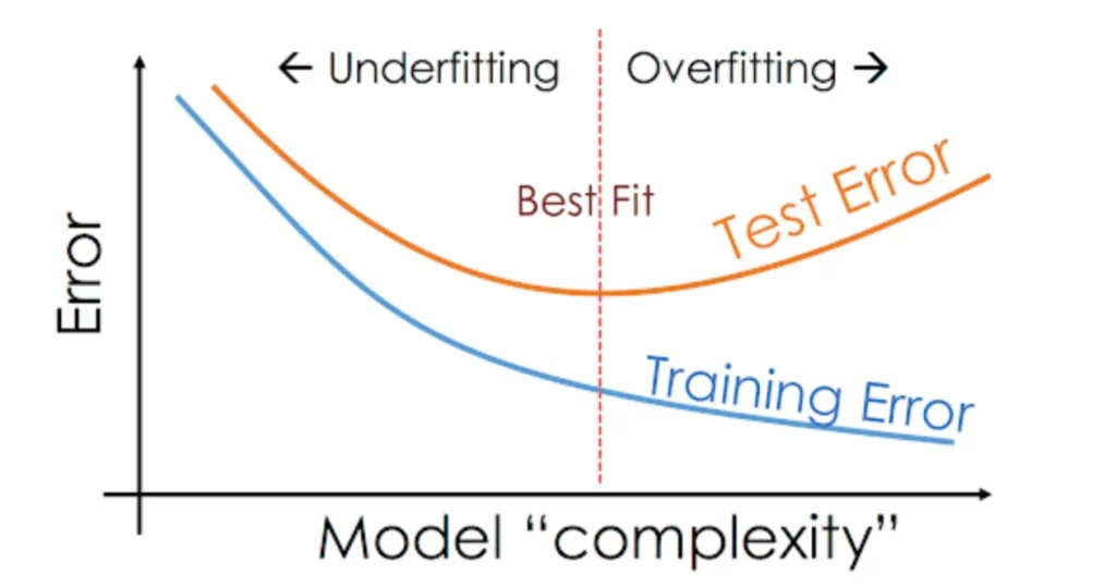
Regarding model complexity, Figure 5 shows the trade-off between having a model that is too simple or too complex. In the case of neural networks, once the hyperparameters of the model (and hence its complexity) are fixed, there is the same trade-off in the number of epochs performed during training.
If not enough epochs are performed, the model will not be able to learn the structure of the data. In this case, the calculated error, both on the training set and on the validation or test set, is relatively high (there is still room for improvement).
Model overfitting
If, on the other hand, the model is overtrained (too many epochs), it will yield minimum error on the training set at the expense of losing ability to generalize. That is, worse results will be obtained for data sets not used for training, such as the validation set or the test set.
Conclusion
As we have seen, for a model as simple as the simple perceptron, there are many variants, such as the choice of the loss function and the activation function, or the stopping criterion. Of course, as in any data science project, good pre-processing of the input data, including cleaning and normalisation, is key to improve our results.
We invite you to continue with our next post The Simple Perceptron: Python Implementation an example of Python implementation of this algorithm, where we study how different simple perceptrons can be combined to form artificial neural networks, with a learning process similar to the one described here, but more complex.
If you found this post useful, we encourage you to see more articles like this one in the Algorithms category of the Damavis Blog and to share it with your contacts so that they can also read it and give their opinion. See you in networks!
