For years, Airflow has been used as a scheduler that allows tasks to be executed at specific times. This was done using cron expressions that specified the exact time an event was to occur.
This approach works well for traditional batch processes. If you want to load dimensions at night, or refresh or load tables periodically, this method is useful and even recommended. However, as architectures evolve and pipelines become more complex, we need to implement different scheduling systems that better adapt to current needs.
In most systems, executing a pipeline isn’t just about a specific time. It depends on various factors, such as the arrival of new data or the completion of another pipeline.
With classic cron-based scheduling systems used to manage this type of pipeline, bottlenecks can occur. Additionally, inelegant patterns may emerge that accumulate failures or delays and base their entire operation on perpetual sensors, creating fragile and inefficient dependencies.
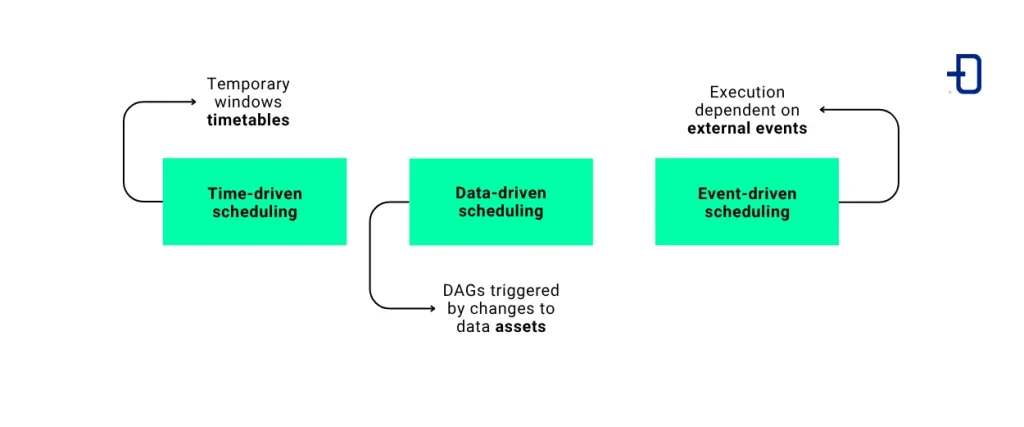
For this reason, Airflow 3 has taken a new approach to how schedulers work. In this version, everything has been structured around three different concepts:
- Time-driven scheduling. This approach is based on time windows defined by timetables.
- Data-driven scheduling. Here, DAGs are triggered when a data asset changes.
- Event-driven scheduling. Execution responds to external events, such as a file modification.
With this in mind, we will explore how scheduling works in Airflow 3 and what its main mechanisms are. We will also analyse different examples and see when it is best to use one or the other.
What is a scheduler in Airflow
Since we’ll be discussing schedulers quite a bit, the first step is to define what they are and what they’re used for. A scheduler in Airflow is a component responsible for deciding when to start a new run of the DAGs available in the system.
It’s important to understand that the scheduler does not execute tasks directly. Its role is to determine when they should run and send them to the appropriate execution system so that workers can process them. Therefore, it is responsible for setting the start time of the DAG and allowing the defined tasks to run.
How scheduling works in Airflow 3
To do this, the scheduler operates in a continuous loop. It analyzes the DAGs and checks whether it should start a run. If the specified conditions are met (whether based on time or other criteria), it generates a new run instance (or, in other words, a new DagRun).
A DagRun is a specific instance of a DAG execution and contains all the information required for its execution. This is key, because each DagRun is associated with a specific data interval. This interval represents the range of data that the DagRun must process. Thus, you can specify which data should be processed and at what point in time, regardless of whether the date in question is the current one or not. For example, a DAG that runs on Monday might be processing data from Sunday or Monday of the previous week.
This is very important because it gives the tool incredible flexibility. By controlling this parameter, you can process any point in time present, past, or, in some cases, future.
Timetables and DagRuns
On the other hand, the element responsible for defining when a new DagRun should be created is the Timetable. Timetables determine both when a new run should start and the data interval associated with it. In other words, the timetable defines the logic that Airflow uses to calculate the next run of a DAG.
However—and this is the key point—Airflow allows you to create runs in response to events other than just time-based ones. It also enables a DagRun to start when a dataset changes, when another process finishes, or when an external event occurs within the system. And this, once again, provides great flexibility.
We’ve already seen the role schedulers play and we understand what DagRuns and Timetables are. Next, we’ll move on to the next point: time-based scheduling using timetables.
Timetable scheduling in Airflow
A timetable defines the logic that Airflow uses to determine when a new DagRun should start and which data range to process. That said, the first thing that comes to mind is setting a specific time using a cron job. However, the reality is that this goes far beyond simply determining a specific time and day. A timetable not only defines when a DAG runs, but also the data interval to be processed during that run.
Using a cron job, we can set up periodic executions over time. As we’ve mentioned, this is particularly significant. Each DagRun is associated with a specific data interval and is bounded by data_interval_start and data_interval_end.
Example of Timetable scheduling
This may not be obvious at first glance, but it is actually very powerful. Let’s look at a use case to see how it works. For example, let’s configure a DAG to run every day at 8:00 AM using a cron expression.
schedule = '0 8 * * *'When you do this, what actually happens is that a DagRun is created at that moment to process the data from the previous interval. In other words, the run scheduled for March 20 at 00:00 will process the data spanning from the start of the 19th to the start of the 20th. Therefore, 03/19/2026 00:00:00 would be the data_interval_start and 03/20/2026 00:00:00 the data_interval_end.
In this way, Airflow is able to completely separate the moment the DAG starts from the data it is processing. This is especially useful when running batch pipelines, as the data is organized into clearly defined windows.
However, despite its advantages, this approach is not always the most appropriate. In many cases, a DAG depends on another process having finished beforehand, as it needs the data that process generates. In these situations, a common solution is to use sensors that point to other DAGs. This can lead to more complex flows, fragile dependencies, and an architecture that is difficult to maintain.
To address this problem, Airflow provides other, more suitable scheduling models, which we will explore below.
Asset-aware scheduling in Airflow
Asset-aware scheduling changes the way DAGs are executed. First, execution is no longer focused solely on the execution time but instead depends on the states of other DAGs in the system. In other words, with this model, you can configure DAGs to run when an asset has been updated. This capability is particularly useful in pipelines where data availability is critical.
What are assets
First and foremost, it is important to define what an asset is. An asset can be a table in BigQuery, a folder in GCS, or any other resource considered a dataset. The key point to keep in mind is that an asset is not a location in and of itself, but rather a representation of how that data fits into the data flow.
This is relevant because a DAG can act as a producer of an asset, causing another DAG—configured for that purpose—to run automatically after a task is executed. This creates a direct dependency based on data rather than one based on time.
Thanks to this, we can eliminate the need to use sensors to coordinate DAGs with one another. Thus, we will move away from fragile time-based dependencies to start reacting to events such as data updates.
Example of asset-aware scheduling
One example could be a dimension load in a data warehouse executed by a DAG, which must necessarily precede a transformation process because the data must be up to date before this point. Using asset-aware scheduling, we can configure the DAG that executes the transformation so that it runs only after the dimension load has finished and the data is therefore up to date. This ensures consistency in the process and guarantees that the final data obtained was generated using up-to-date sources.
To better understand this behavior, let’s look at a practical example. On one hand, this would be the producer DAG, which would mark the asset as updated so that the consumer DAGs can run.
master_ingestion_ready = Dataset("master_ingestion_ready")

def run_ingestion():
    print("Master ingestion completed")

dag = DAG(
    dag_id="producer_dag_1",
    start_date=pendulum.datetime(2026, 1, 1, tz="UTC"),
    schedule=None,
    catchup=False,
)

produce_asset = PythonOperator(
    task_id="run_ingestion",
    python_callable=run_ingestion,
    outlets=[master_ingestion_ready],
    dag=dag,
)
On the other hand, the consumer DAG would look like this.
master_ingestion_ready = Dataset("master_ingestion_ready")

def run_transformation():
    print("Transformation started after ingestion")

dag = DAG(
    dag_id="consumer_dag_2",
    start_date=pendulum.datetime(2026, 1, 1, tz="UTC"),
    schedule=[master_ingestion_ready],
    catchup=False,
)

consume_asset = PythonOperator(
    task_id="run_transformation",
    python_callable=run_transformation,
    dag=dag,
)
As you can see, the first DAG acts as the asset’s producer, indicating that the data has been updated following its execution. On the other hand, the second DAG is configured to run whenever that asset changes. This allows for the establishment of a direct data-driven dependency without the need for sensors.
Finally, it is important to note that, although this strategy has many advantages over Timetable scheduling, in some cases it may be necessary to combine this approach with periodic executions to ensure consistency or to cover certain situations where no updates occur. To this end, Airflow provides other mechanisms, such as the one we will discuss below.
What AssetOrTimeSchedule is and how it works in Airflow
AssetOrTimeSchedule is characterised as a hybrid model between timetable scheduling and asset-aware scheduling. It allows a DAG to run either when an asset is updated or when a time-based condition is met.
This type of scheduling is especially useful if the goal is to ensure the pipeline runs under any circumstances—whether because data has been updated or because a specific point in time has been reached. This prevents unprocessed data from accumulating in cases where no updates occur during a given period.
In practice, this means that, thanks to AssetOrTimeSchedule, a DAG can run when an asset has been updated. However, it can also run automatically at a specific point in time. This ensures data consistency and prevents potential gaps in which information is missing.
An example of using AssetOrTimeSchedule would be as follows.
master_table_ready = Dataset("master_table_ready")

def run_reporting():
    print("Reporting pipeline started")

dag = DAG(
    dag_id="reporting_dag",
    start_date=pendulum.datetime(2026, 1, 1, tz="UTC"),
    schedule=AssetOrTimeSchedule(
        timetable=CronTriggerTimetable("0 8 * * *", timezone="UTC"),
        assets=[master_table_ready]
    ),
    catchup=False,
)

run_report = PythonOperator(
    task_id="run_reporting",
    python_callable=run_reporting,
    dag=dag,
)
In this case, the DAG will run in two different situations: either when the master_table_ready asset has been updated, or when the execution scheduled by the timetable at 8:00 a.m. occurs. This ensures that the pipeline runs in either case.
Therefore, AssetOrTimeSchedule, rather than providing a new triggering system, offers a kind of extra safety mechanism for asset-aware scheduling. This allows us to design pipelines that are much more fault-tolerant and adapted to different processing scenarios.
Event-driven scheduling in Airflow 3
Finally, we will look at a new method introduced in Airflow 3, Event-driven scheduling. Its main advantage is that it provides a new execution model that reduces reliance on time or data availability. In this case, it is triggered when a series of external events occur.
Thanks to this, Airflow allows for the construction of pipelines that are much more responsive than before. Now, they are capable of responding to situations the moment events occur.
What are Airflow events
However, it is important to define what an event is. An event can be any signal indicating that a process should be initiated. For example, the arrival of certain files in GCS, a change to a manifest, or the appearance of a new item in a queue system, among others.
As you can see, there is a wide variety of elements that can trigger a pipeline. Thanks to event-driven scheduling, instead of periodically checking whether certain conditions are met, the DAG reacts when one of these events occurs.
To make this possible, Airflow has introduced a trigger-based architecture. With this architecture, it is possible to manage events without tasks having to run constantly while waiting for a condition to be met.
Deferrable operators
To fully understand this section, it is important to know about deferrable operators. The sensors previously implemented in Airflow performed continuous pulls to verify whether the specified condition had been met. In contrast, these operators can pause their execution and wait for the trigger to instruct them to run. Once this occurs, the process resumes and the task is executed.
This is especially useful when system resources are limited. It shifts from having a sensor continuously pulling data, waiting for a given condition to be met, to having a trigger system that only executes once the event occurs.
Example of event-driven scheduling with Kafka
To demonstrate the wide range of applications for this new execution model, we will look at two examples. First, we will show how to use it to trigger the DAG when a specific event occurs (such as data arriving in a Kafka queue). In the second example, we will examine how it can be applied to a specific task.
First, we’ll see how the DAG would be implemented to continuously listen for an external event stream using the new Asset Watchers. This allows streams to be defined as Assets instead of relying on batch processes. By associating a watcher with them, they delegate the task of triggering actions in the background to the scheduler.
In this way, the DAG no longer depends on the time at which it must run. Now, it remains inactive and does not consume resources, waiting for the event that will trigger its execution to occur.
An example of a structure that waits for a Kafka event to occur would be the following:
trigger = MessageQueueTrigger(
    queue="kafka://localhost:9092/airflow_example_topic",
    apply_function="include.kafka_trigger.apply_function",
)

kafka_topic_asset = Asset("kafka_topic_asset",
    watchers=[AssetWatcher(name="kafka_watcher", trigger=trigger)]
)

dag = DAG(
    dag_id="kafka_event_driven",
    start_date=pendulum.datetime(2026, 1, 1, tz="UTC"),
    schedule=[kafka_topic_asset],
    catchup=False,
)

load_to_bq = GCSToBigQueryOperator(
    task_id="load_to_bq",
    bucket="data-bucket",
    source_objects=["incoming/master_data.csv"],
destination_project_dataset_table="project_id.datawarehouse.master_data",
    source_format="csv",
    dag=dag,
)
As can be seen in this example, the DAG does not require an internal waiting mechanism. The scheduler handles active listening, with the resulting advantage that the DAG does not start until the event has occurred.
Use case for event-driven scheduling with BigQuery
On the other hand, an example of its use in a specific task could be loading dimensions from GCS to BigQuery. Until now, the operator performing the load had to have previously set up a sensor that blocked a worker by detecting whether the file had been changed. If this event occurred, the pipeline could continue. Thanks to deferrable operators, the pipeline can efficiently wait for, say, a manifest to be modified, freeing up resources until this happens.
To ensure the DAG does not depend on manual or external triggering and maintains the deferrable approach, the ideal solution in modern versions of Airflow is to combine a hybrid approach. For example, a traditional cron job with a deferrable sensor.
An example of this scenario would be as follows:
dag = DAG(
    dag_id="gcs_to_bigquery_event_driven",
    start_date=pendulum.datetime(2026, 1, 1, tz="UTC"),
    schedule="30 8 * * *",
    catchup=False,
)

wait_for_file = GCSObjectExistenceSensor(
    task_id="wait_for_file",
    bucket="data-bucket",
    object="incoming/master_data.csv",
    deferrable=True,
    dag=dag,
)

load_to_bq = GCSToBigQueryOperator(
    task_id="load_to_bq",
    bucket="data-bucket",
    source_objects=["incoming/master_data.csv"],
destination_project_dataset_table="project_id.datawarehouse.master_data",
    source_format="csv",
    dag=dag,
)

wait_for_file >> load_to_bq
As we can see, this DAG does not rely on a sensor that constantly polls and blocks a worker. Its wait task is triggered when it detects that the file has arrived in GCS. This allows the system to consume far fewer resources. Therefore, this structure is particularly useful in event-driven architectures, where pipelines must run when changes occur in the system.
However, we must be careful about how this new model is used. If our pipeline does not require this level of reactivity, we may end up with overly reactive pipelines that are much harder to maintain—pipelines that could just as easily be executed using traditional datasets (assets) or timetables.
Conclusion
As we have seen, Airflow schedulers go beyond the time-based execution of DAGs. Furthermore, they are an integral part of the pipeline architecture itself. This allows us to adapt our processes to different scenarios and needs.
On one hand, we’ve seen how Timetable scheduling focuses on traditional batch processes. Meanwhile, asset-aware scheduling focuses on data availability, and event-driven scheduling focuses on reacting to external events. All of them offer different approaches to efficiently orchestrating our workflows.
A clear understanding of their differences is crucial and enables the design of robust, maintainable, and scalable pipelines. In many cases, this is what distinguishes a mediocre system from an excellent one.
In short, Airflow 3 not only expands scheduling capabilities by adding event-driven scheduling; it also changes the way we need to think when designing our pipelines. Now, we must not only understand the workflow that will be executed, but we must also always keep in mind whether we want our system to run at specific times or react to specific events that we define.
So much for today’s post. If you found it interesting, we encourage you to visit the Software category to see similar articles and to share it in networks with your contacts. See you soon!
