Optimal Pricing in a hotel demand model

Revenue management (RM) can be defined as a set of techniques focused on analyzing consumer behavior with the purpose of obtaining the highest possible profit. In general, understanding how customers’ willingness to buy a certain good responds to this good’s price is key. In this way, one can estimate how demand will be affected by a shift in price, and thus take actions in order to maximize revenue.

Focusing on the hotel context, the problem of finding the relation between price and demand might become highly involved as multiple actors come into play. Naturally, there might be different types of customers which respond differently to variations in price. For example, leisure customers tend to be pretty price elastic, meaning that a variation in price may substantially affect their willingness to make a reservation. This is in contrast to business customers who are in general more price inelastic, as they are often refunded for their expenses and thus do not mind booking a room at a higher rate.

In addition to different types of customers, one might also consider different types of rooms, with different prices associated with them. On top of that, we could find different customer behavior depending on the season or the day of the week, among other factors. 

In this post, for illustration purposes, we will stick to a simple setting in which we do not consider different types of customers, seasons, or rooms. Our purpose is not to infer the behavior of the demand from some given data set. Instead, we below define a simple model for demand, and we will focus on finding an optimal pricing strategy given this model.

A simple hotel demand model

Let us assume the following scenario: we are a hotel manager who needs to set room prices up to T days in advance. For example, T = 356 in case we allow for reservations up to one year before the check-in date. The price for a given date of stay is set at the beginning of each booking day and is maintained during the whole day.

At the beginning of the next day we might choose a different price for the same arrival date, and the same process is repeated until the arrival date, inclusive. Consider that our goal is to maximize total profits obtained from room reservations the day after arrival (as we allow for reservations on arrival day itself). Naturally, in order to set a pricing strategy, we need to have some knowledge on how the number of rooms demanded for a given date of stay, or demand, will respond to a price change. 

A common approach in the literature about hotel demand estimation is to consider the demand for rooms as a random variable. This quantity is regarded as the combination of the individual decisions of a number of potential customers looking for accommodation in a market where our hotel has presence. This number of individuals, which we refer to as the market arrivals, or simply arrivals, is denoted by 𝐴.

Let us consider a fixed check-in date for which we want to maximize profits obtained from room reservations. In general, we will index the variables in our model with 𝑡, which denotes the number of days between the current day and the arrival date. Suppose the expected number of arrivals at time 𝑡 (this is, 𝑡 days before arrival), denoted by 𝑎_𝑡, was found to increase linearly as we approach arrival day (or 𝑡 approaches zero). Consider that the probability distribution of the number of arrivals 𝐴_𝑡 at a given advance day 𝑡 is given by:

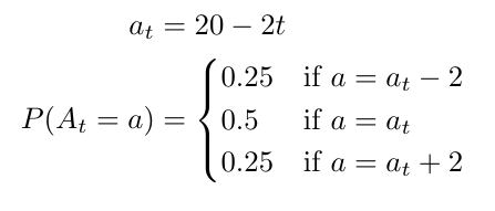
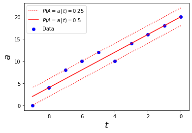
when 𝑡 ∈ [0, 9] and 𝑃 (𝐴_𝑡 = 0) = 1 otherwise.  This means that no customers look for accommodation in our market before 9 days prior to arrival, and from 𝑡 = 9 onwards the potential number of customers increases linearly. For instance, at 𝑡 = 9 we have an expected number of arrivals 𝑎₉ = 2 , so there is a 25% chance that we have 𝐴₉ = 2 – 2 = 0 new market arrivals, a 50% chance that are 𝐴₉ = 2 new arrivals, and a 25% chance we have 𝐴₉ = 2 + 2 = 4 new arrivals. At arrival day (𝑡 = 0), we have 𝑎₀ = 20, so the possible values for 𝐴₀ are 18, 20 and 22, with respective probabilities 25%, 50% and 25%. Of course, in general the arrival function will be way more complex, but as we said, this example is simplified for illustration purposes. Figure 2 shows how the arrival curve looks like.

Once we know the distribution of arrivals (the number of potential customers in our market at a given day), let us calculate the distribution of the actual demand. It seems safe to assume that each individual makes their decision independently of the rest, and they will choose whether to book a room at our hotel or not according to some utility value.  Of course, these utility values may vary among customer segments, and even within these groups, as each person has their own conception of utility. Again, by simplicity, let us assume in this model that the probabilities that each of the potential customers chooses our hotel are equal, and let us call this common value the choice probability. With this assumption, demand follows a binomial distribution, the size parameter of which is the number of market arrivals, and the probability parameter is the choice probability.

The choice probability can be formally defined as follows. Let 𝑋 be a Bernoulli random variable taking values 1 or 0 depending on whether a given customer in the market decides to book a room in our hotel or not, respectively. Then, the choice probability is just the probability of 𝑋 equaling 1. Naturally, this probability depends on the price 𝑝 we set and potentially other factors, such as the competitors’ prices and other less measurable quantities like the customer’s perception of quality of the different hotels. For this example, consider the naive choice probability

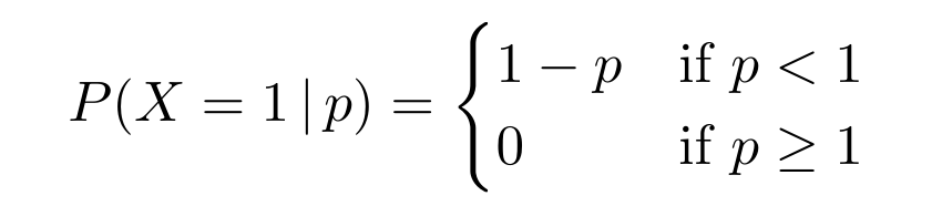
which fixes an upper bound for price. Indeed, if 𝑝 ≥ 1 the choice probability is zero, which means that no one books a room at our hotel, and as 𝑝 approaches zero we get a higher probability that our hotel is chosen.

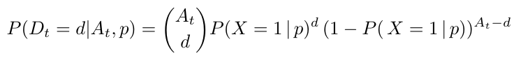
Once we know the common choice probability and the number of market arrivals at the present day 𝑡, the number of rooms demanded 𝐷_𝑡 can be calculated as a binomial distribution as follows:

However, in practice, the number of arrivals 𝐴 will be unknown, since we must be able to estimate demand at a given day 𝑡 before this day arrives. For instance, we could get a demand of 10 rooms at day 𝑡 as a result of 20 customers arriving to the market, a half of which choose to book at our hotel, or as the result of a total arrival of 100 customers with only a tenth of the market share. Both scenarios, with their respective probabilities, must be taken into account in order to calculate the demand probability.

Therefore, we have to rewrite the above expression taking into account that the number of arrivals as a function of 𝑡 is itself stochastic, with the probability distribution defined above. Thus, the probability of having a demand d at day 𝑡 given that we set a price 𝑝 is given by

where a spans over all possible values for the number of potential customers at day 𝑡.

We already know the distribution of the number of rooms demanded at any given advance time 𝑡 when a price 𝑝 is set. However, a distinctive characteristic of the hotel demand scenario is that the quantity of the goods provided, i.e. the number of rooms, is bounded above by the total capacity of the hotel, call it . Therefore, the realized demand (number of rooms actually booked) might not equal the number of rooms demanded when there are not enough available rooms.

In particular, let 𝑛_𝑡 be the occupancy (number of rooms already booked for a given date of stay) at the beginning of day 𝑡, and let 𝑑_𝑡 be the number of rooms demanded during day 𝑡.  Following a strict overbooking policy, in which we do not allow for any excess in capacity, the expressions for the realized demand 𝑑_𝑡 and for the occupancy on the next day 𝑛_𝑡-1 will be given by

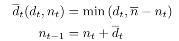
In other words, we will allow all the reservations until we reach full capacity. 

It is worth noting that in most real world scenarios, hotels also allow for cancellations in advance. These cancellations would leave room for new reservations, thus slightly modifying our model. In particular, let 𝑐_𝑡 be the number of bookings cancelled at day 𝑡, the realized demand would become . If cancellations could be made, one could also allow for a given level of overbooking in order to ensure full occupancy.

Following the simplicity principle, we do not allow for cancellations nor overbooking in this model. However, they might be added with little overhead.

Optimal pricing strategy: the value function

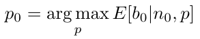
Remember we said our goal is to maximize the total benefits obtained from room reservations the day after arrival. Let  𝑏_𝑡 be the benefits obtained from reservations made a number of days 𝑡 before the arrival day. When we find ourselves at arrival day ( 𝑡 = 0 ), with a given occupancy 𝑛₀,  we just need to maximize the expected benefits on arrival day 𝑏₀. Naturally, profit obtained from last day reservations will depend on the price set during this day. In particular, we want to choose the price 𝑝₀ which maximizes the expected benefit

As long as cancellations are not allowed, the benefit obtained at any day 𝑡 is just the product between the number of rooms booked the realized demand , and the price 𝑝_𝑡 set,

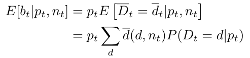
Note that the realized demand is a random variable as it depends on the quantity demanded, which is itself a random variable whose distribution is given by Equation 1. Thus, we can find the expected value of the realized demand given a time 𝑡, a price 𝑝_𝑡 and a current occupancy 𝑛_𝑡 by summing over all its possible values weighted by their respective probabilities. Then, for each possible value of the price 𝑝_𝑡 set at day 𝑡, we can calculate the expected daily profit 𝑏_𝑡 by using the simple formula

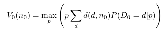
Let us assume that we find ourselves a number of days 𝑡 before arrival, and define the value function 𝑉_𝑡 (𝑛_𝑡) as the maximum of the total expected benefit from now on, which is achieved by setting an optimal price given that the current occupancy is 𝑛_𝑡. As we argued, if we are at arrival day ( 𝑡 = 0 ), the value function is just the value of the expected benefits on the current day, for an optimal choice of price. Therefore, using the previous formula we can write

However, when setting prices a number of days ahead of time, our goal is not to maximize the current day’s benefit, but the overall benefit in the long run. For instance, suppose demand is low at the moment but we have the certainty that it will boost as arrival day gets closer. In this situation, if we already have an acceptable occupancy rate, we might be interested in setting a high price and giving up some benefit at the moment in order to keep available rooms for last moment reservations, which we might be able to sell at a higher rate.

The expected benefit from now on will thus depend on the benefit we expect at future days ( 𝑡’ < 𝑡 ), and this gives us a way to define the value function recursively as

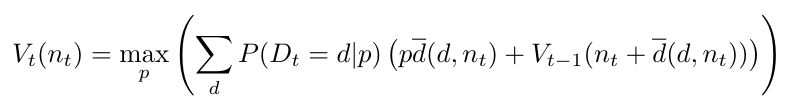
This is, the maximum expected benefit in the long run will be achieved by the price which maximizes the expected value of the sum between today’s benefits, expressed by the term, and the maximum expected benefits from tomorrow on. This is represented by tomorrow’s value function , where the argument represents tomorrow’s occupancy given that we have a demand 𝑑 today.

We can see that in order to find the value of 𝑉_𝑡 (and thus the optimal price 𝑝_𝑡 to be set at the given day 𝑡 > 0) , we need to calculate the value function for the upcoming day 𝑉_𝑡-1 , which will in turn require the calculation of 𝑉_𝑡-2 , and so on.

In a previous post we talked about how dynamic programming comes in handy in such recursive problems in order to avoid repetitive calculations. We will show in an upcoming post how to find the optimal price by solving the recursive value function using a dynamic programming approach. In the meantime, we encourage you to visit the Data Science category of the Damavis blog and read articles similar to this one.

If you found this post interesting, we encourage you to share this article on social media. Don’t forget to mention us to let us know what you think (@DamavisStudio) , see you networks!