Dynamic programming and the Fibonacci series

Dynamic programming

Dynamic programming (DP) is a computer programming method which consists in breaking down a complex problem into smaller problems, usually in a recursive way. Then, these problems are solved one at a time, typically storing the already computed results so as to avoid computing them more than once.

Dynamic programming and the Fibonacci series

A paradigmal example of a problem which can be solved using DP consists in finding the n-th term of the Fibonacci series. The Fibonacci series is defined recursively in the following way:

That is, in order to calculate the value of the n-th term of the series F_𝑛, we need to know the previous two terms. Thus, a simple recursive approach might be used to solve the problem.

def fibonacci_recursive(n):
    if n == 0 or n == 1:
        return 1
    else:
        return fibonacci_recursive(n-1) + fibonacci_recursive(n-2)

While correct, this implementation is extremely inefficient. For example, if we try to calculate the fourth value of the series by calling

fibonacci_recursive(4)

we do indeed get the correct value F₄ = 4 . However, this function call with 𝑛 = 4 subsequently causes two recursive calls to the function with arguments 𝑛 -1 = 3 and 𝑛 – 2 = 2 . These, in turn, trigger further recursive calls in order to calculate their value, and so forth until reaching the base cases F₀ and F₁.

The following diagram shows the flow used to compute the previous value, where each box represents a function call.

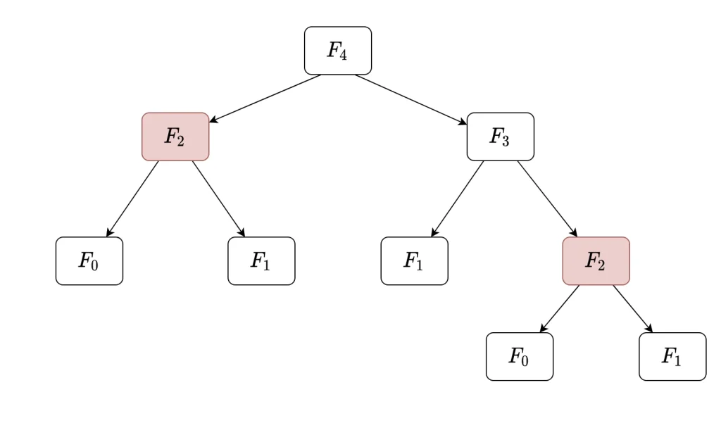
As we can observe, the function is run a total of 9 times, and there are 4 calculations of non-trivial (that is, not a base case) terms: one for F₄, one for F₃ and two for F₂.  Indeed, the red boxes show that the non-trivial term F₂ is needlessly computed twice: once in the calculation of F₄ in the upper level, and again in the calculation of F₃. 

Given this setting, the following natural question arises: how can we avoid repetitive computations to calculate the value of F₄? As you might have guessed, this is where dynamic programming comes into play.

We already noted that in order to calculate the n-th element of the series we need to calculate the two previous terms. By induction, it follows that we need to calculate all  the terms of the sequence up to the n-th element in order to calculate its value. Given that we need to compute all the terms of the sequence, consider the following approach: we will start by setting the trivial base cases, and then starting from the first non-trivial term, we will iteratively calculate the following element using the previous two values.

The key point is that each time we calculate a value, we will keep this value in our program’s memory, so we can reuse it whenever it is necessary in the future. In the Fibonacci series example, the first non-trivial value we will calculate is F₂ . Note that, once this value is computed, we will use it in order to calculate the following term of the series, F₃ = F₁ + F₂ , and also in the next one, F₄ = F₂ + F₃ . Therefore, despite being used twice, by saving it in memory we can compute it only once.

Implementation example of a dynamic programming approach

Here is an example of the implementation of a dynamic programming approach to solve the problem of finding the n-th term of the Fibonacci series:

import numpy as np

def fibonacci_dp(n):
    if n == 0 or n == 1:
        return 1
    
    last_value = 1
    current_value = 1
    for i in range(n-1):
        aux_value = current_value
        current_value += last_value
        last_value = aux_value
        
    return current_value

Although this function looks more complex than the fibonacci_recursive above, it is in fact much more optimal. In particular, it involves only n-1 non-trivial calculations which correspond to the calculation of terms F₂ , F₃ , … , F_𝑛 , one time each. This is in contrast with the naive recursive approach, which involves a number of calculations which grows exponentially with 𝑛 .

For example, in the case of calculating F₅, only 4 calculations are needed, while 7 would be needed using the recursive function. For F₁₀ , just 9 calculations are used instead of 88.  If we calculated F₅₀ , using the DP approach we would need just 49 sums, while the recursive approach would require 20,365,011,073 calculations!

Conclusion

This simple example illustrates the importance of choosing an efficient way to tackle a problem, even when there are different alternatives yielding the same result. This is particularly key when the problem has a recursive nature requiring the use of previously computed values. In this case, we saw that by just storing these values using a dynamic programming approach, overhead is dramatically reduced, especially as the number of nested calculations increases.

In future posts we will show how to apply a dynamic programming model to solve the problem of pricing in hotels. In particular, we will use it for calculating the optimal price to be set a number of days before the date of stay, in order to maximize benefits in the long run.

In the meantime, we encourage you to visit the Algorithms category of the Damavis blog for more articles similar to this one.

If you found this post useful, we invite you to share it with your contacts . See you in social networks!