

Pyspark ML is an Apache Spark module used to train predictive models on DataFrames. Its purpose is not limited to that; it also enables a range of other machine learning-oriented operations. For example, imputing missing values or standardising variables, which greatly streamline the entire training process.
One advantage of Pyspark ML over other machine learning libraries is its ability to train models on very large datasets. Furthermore, this can be done in a distributed manner. This plays a crucial role when dealing with a large volume of data for training, as PySpark ML allows processing to be distributed across multiple nodes. This simplifies the tasks of preparing variables, generating predictions, and evaluating results within the same workflow and in an environment designed to scale as needed.
In this article, we’ll explore a practical introduction to training models with PySpark ML. We’ll also examine the basics of transformers, estimators, and pipelines, which form the foundation for working in a reproducible and organised manner on machine learning projects with Spark.
Spark MLlib vs Spark ML
Before you start training models with PySpark, it’s important to clear up a common misconception. pyspark.mllib is not the same as pyspark.ml. Although they may seem to work the same way, there are differences between them that you should be aware of.
On the one hand, pyspark.mllib is the legacy API based on RDDs, which is now considered obsolete for most use cases. On the other hand, pyspark.ml is the modern API, built on DataFrames, and is the recommended option for developing machine learning pipelines in Spark.
This difference is not just a name change. Working with DataFrames allows for better integration of preprocessing, variable preparation, model training, and evaluation within pipelines. Therefore, in this article, we will focus on pyspark.ml, which is the current and most practical way to build machine learning models with PySpark.
Training workflow in PySpark ML
The training process in PySpark ML, just as in other machine learning libraries, does not consist solely of selecting an algorithm, executing a method, and obtaining a prediction. To build a model that generates useful results, you need to follow a series of ordered steps. This makes it easier to prepare the data, train the model, and then verify whether it is truly capable of generalising to information it has not seen before.
Typically, the starting point is a Spark DataFrame containing the raw data you want to work with. Before using this data in a model, an initial data cleaning and preparation phase is necessary. At this stage, various operations can be performed. For example, removing duplicate records, correcting data types, handling null values, discarding invalid records, or creating new variables from existing columns.
Before using this data to train a model, situations such as the following may arise:
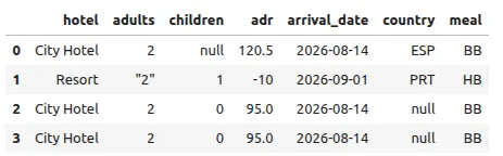
For example, from a column containing a date, new variables such as the day of the week, the month, or the year could be generated. Totals, tenure, averages, or any other variable that could provide relevant information to the model could also be calculated.
Data and variable transformations
However, it is important to distinguish between general transformations that can be applied directly to the data and those that require learning information from the data. For example, removing duplicates or extracting the month from a date does not involve learning any statistical patterns. In contrast, calculating averages to fill in missing values, scaling variables, or converting categories into indices may depend on the data distribution.
This distinction is crucial because transformations that learn from the data should not be tuned using the entire dataset. If information from the test set is used during training—even indirectly—it can lead to data leakage. As a result, the model might appear more accurate than it actually would be when working with new data. This is a consequence that must be avoided at all costs.
For this reason, after performing an initial cleanup, the DataFrame must be split into a training set and a test set. The training set will be used to fine-tune both the transformations that need to learn from the data and the algorithm itself. The test set, on the other hand, will be reserved for evaluating the model’s performance once training is complete.
Once the data has been split, the next step is to transform the variables into the format expected by Spark ML. Most algorithms do not receive each input variable as a separate column; rather, they expect a single vector column that groups all the features used by the model. By convention, this column is usually called features, although another name may be used if deemed necessary. However, the algorithm must always be configured correctly to account for this.
Types of variables
How this column is prepared depends on the type of variables. While numerical variables can be used directly if they are clean, categorical variables must be transformed into a numerical format using tools such as StringIndexer and OneHotEncoder. After these adjustments, all variables are combined using, for example, VectorAssembler, which generates the feature vector used by the model.
In supervised learning problems, it is also necessary to have a target variable—that is, the column containing the outcome we want the model to learn to predict. This column is typically called a label, although, as with features, any name can be used as long as it is properly configured.
The target variable will depend on the type of problem you want to solve. In classification, it could represent, for example, whether a customer makes a purchase, whether a transaction is fraudulent, or which category a record belongs to. In regression, it could represent a continuous value, such as the price of a home, the amount of a sale, or the time required to complete a task.
Defining the algorithm
Once the necessary transformations have been defined, the features field has been prepared, and the target variable has been established, you can define the algorithm to be used during training. At this point, PySpark ML includes various models for classification, regression, clustering, and dimensionality reduction, among others. Therefore, it is important to know which one is most appropriate for each use case.
Training is performed using the fit() method. This method takes the training DataFrame and generates a trained model. During this process, the algorithm analyses the relationship between the input variables and the target variable and learns the internal parameters needed to make predictions.
After training the model, it can be applied to the test set using the transform() method. The result of this operation will be a new DataFrame that retains the original columns and incorporates those generated by the model. These columns include, among others, a new one typically called prediction, which will contain the prediction obtained for each record.
Results and pipeline
The final step involves evaluating the results obtained. To do this, the model’s predictions are compared with the actual values of the target variable. The metrics used depend on the type of problem. Typically, for classification problems, it is common to use metrics such as accuracy, precision, recall, F1-score, or area under the ROC curve. On the other hand, for regression problems, RMSE (Root Mean Squared Error), MAE (Mean Absolute Error), or R² (coefficient of determination) are typically used.
Finally, it is important to understand that, although all of these steps can be executed independently, PySpark ML allows you to group many of the transformations and the algorithm itself into a pipeline. The pipeline allows you to define the entire workflow as an ordered sequence of stages and tune it using only the training data. This is particularly useful because, once training is complete, that same workflow can be applied to the test set or to new data, ensuring that exactly the same transformations are performed.
In summary, the training process is quite demanding and requires performing several steps in a specific order to find a particular function. However, that’s not all. It’s important to understand other fundamental aspects of PySpark ML, such as how to use transformers, estimators, pipelines, predictive models, and evaluation tools.
Data format in PySpark ML
PySpark ML works directly with Spark DataFrames, so there is no need to convert the data to external structures before training a model. However, the algorithms expect the DataFrame to follow a specific structure, particularly with regard to the input variables and the variable to be predicted.
In addition, you must verify that the columns have compatible data types. Numeric variables must be correctly converted and should not contain null values, infinite values, or invalid data. Categorical variables also cannot be directly incorporated into the vector. Therefore, as mentioned earlier, they must first be transformed using components such as StringIndexer and, when necessary, OneHotEncoder.
As you can see, Spark ML requires that the variables used by the model be correctly typed, transformed, and grouped into a single vector column. This common structure allows the various algorithms and components of PySpark ML to connect with one another in a consistent manner.
Transformers in PySpark ML
Transformers are PySpark ML components that take a DataFrame, apply an operation to its data, and return a new DataFrame with the transformed or added columns. To perform this operation, they use the transform() method.
It is important to note that a transformer does not directly modify the original DataFrame, since Spark DataFrames are immutable. Instead, it generates a new one that preserves the existing columns and incorporates the result of the transformation.
Using VectorAssembler
A great example illustrating the use of a transformer is VectorAssembler, which allows you to group several numeric columns into a single vector column—which, as mentioned earlier, are often called features:
from pyspark.ml.feature import VectorAssembler

assembler = VectorAssembler( inputCols=["nombre", "edad", "ingresos"], outputCol="features" )

df_transformado = assembler.transform(df)
In this case, VectorAssembler does not need to learn anything from the data. It simply takes the columns we’ve specified and combines them according to a rule we’ve defined. For this reason, it can be used directly via the transform() method.
There are also transformers designed to modify columns, generate new variables, or apply pre-trained models. In fact, when an algorithm is trained using the fit() method, the result is a model that also functions as a transformer. This model can take new data and add columns such as prediction or probability.
So, as you can see, there are two common types of transformers in PySpark ML. On the one hand, there are those that apply operations directly to the data (such as VectorAssembler or Tokenizer). On the other hand, there are trained models, which transform a DataFrame by generating predictions based on the patterns learned during training. In both cases, they take a DataFrame as input and return another one using the transform() method without needing to learn parameters at that moment.
As we’ll see in the next section, this is the main difference between transformers and estimators, which must first analyse the data using fit() to generate a transformer model.
Estimators and trained models
Estimators are PySpark ML components that need to analyse a dataset to learn a set of parameters before performing a transformation. Unlike transformers, they are not applied directly using the transform() method; instead, they use fit() to fit the data and generate a trained model as a result.
There are several estimators that are commonly used. For example, StringIndexer is an estimator because it needs to iterate through the data to identify the existing categories so it can assign a number to each one. On the other hand, StandardScaler is used to standardise numerical variables based on statistics such as the mean and standard deviation. This allows us to transform their values so they operate on a comparable scale, preventing some variables from carrying more weight than others simply because they have larger values.
StringIndexer and LogisticRegression()
Predictive algorithms—such as logistic regression, decision trees, and linear regression models—are also estimators. Let’s look at an example.
from pyspark.ml.feature import StringIndexer
indexer = StringIndexer(
    inputCol="ciudad",
    outputCol="ciudad_indexada"
)
modelo_indexador = indexer.fit(df_train)
df_transformado = modelo_indexador.transform(df_train)
In this example, StringIndexer is the estimator, and model_indexer is the trained model obtained after calling the fit() method. The estimator defines how the learning process will take place, while the model contains the learned information and can later be applied to other DataFrames as just another transformer using transform().
Similarly, we can do the same with a predictive algorithm such as LogisticRegression(). Let’s look at another example below:
from pyspark.ml.classification import LogisticRegression

estimador = LogisticRegression(
    featuresCol="features",
    labelCol="label"
)

modelo = estimador.fit(df_train)
predicciones = modelo.transform(df_test)
In this case, LogisticRegression represents the algorithm that has not yet been trained. When the fit() method is run on the training set, a fitted logistic regression model is generated that already contains the learned parameters and functions as a transformer capable of generating predictions.
It is important that estimators be fitted using only the training data. If components such as StringIndexer or StandardScaler are also trained using the test set, information will be incorporated that should remain unknown during training. This situation is highly undesirable, as it can lead to an overly optimistic evaluation of the model.
Therefore, as we have seen, an estimator takes a DataFrame via fit() and returns a trained model. That model then behaves as a transformer and can be applied via the transform() method to the training set, the test set, or new data. This relationship between estimators, models, and transformers is one of the foundations upon which PySpark ML pipelines are built.
Predictive models
Now that we’ve seen the difference between estimators and transformers, the next step is to discuss predictive models. However, first and foremost, it’s important to understand what they are. Predictive models are machine learning algorithms that analyse training data to learn the relationship between the input variables and the target variable. Once trained, they can apply the learned patterns to new data and generate a prediction for each record.
In PySpark ML, predictive models are initially defined as estimators. This means that, before they can make predictions, they must be fitted using the fit() method with a training DataFrame containing the features column and the target variable.
from pyspark.ml.classification import LogisticRegression

algoritmo = LogisticRegression(
    featuresCol="features",
    labelCol="label"
)

modelo = algoritmo.fit(df_train)
In this example, LogisticRegression represents the algorithm before it has been trained, while the model variable contains the resulting predictive model after analysing the data with fit().
As explained earlier, once trained, the model functions as a transformer and can be applied to the test set or to new data using the transform() method.
predicciones = modelo.transform(df_test)This new DataFrame not only retains the original columns but also adds a new column—typically called prediction —that contains the result calculated by the model. Additionally, some classification algorithms generate extra columns, such as probability or rawPrediction. These columns provide the score or probability assigned to each class.
Classification and regression models
It is important to note that the predictive models that can be used in PySpark ML can be broadly divided into two categories: classification models and regression models.
Classification models are used when the target variable represents a category. For example, determining whether a customer will make a purchase, whether a transaction might be fraudulent, or which group a record belongs to. In this case, some of the algorithms that can be used include LogisticRegression, DecisionTreeClassifier, and RandomForestClassifier, among others.
On the other hand, regression models are typically used when the goal is to predict a continuous numerical value. For example, the price of a home, the amount of a sale, or the duration of a service. Among the most notable PySpark ML algorithms are LinearRegression, DecisionTreeRegressor, and RandomForestRegressor.
Model selection is one of the most important aspects of prediction. Each algorithm has different characteristics and may perform better or worse depending on the volume of data, the type of variables, the relationships between them, and the objective of the problem. For this reason, it is common practice to train and evaluate different models before selecting the one that yields the best results. This ensures that the model ultimately chosen is truly the one that produces the best results based on the data.
Evaluating results
Now that the model has been trained and predictions have been generated for the test set, the next step is to evaluate the results obtained. This phase is key to the entire process, as it allows us to verify whether the model has learned useful patterns and whether it is capable of generating accurate predictions on data not used during training.
As we have seen, applying the transform() method to the test set yields a new DataFrame containing both the actual values of the target variable and the predictions made by the model. Therefore, evaluation consists primarily of comparing the label column with the prediction column.
predicciones = modelo.transform(df_test)

predicciones.select(
    "label",
    "prediction"
).show()
However, manually reviewing a few predictions is not enough to determine whether a model is working correctly. To measure its performance objectively, it is necessary to use evaluation metrics. These metrics will depend primarily on whether we are working with a classification problem or a regression problem.
Metrics for classification problems
In classification problems, the goal is to predict a category. For example, you might try to determine whether a customer will make a purchase, whether a transaction is fraudulent, or whether an email is spam. In these cases, PySpark ML provides evaluators such as BinaryClassificationEvaluator and MulticlassClassificationEvaluator.
One of the best-known metrics is accuracy, which indicates what proportion of the model’s predictions are correct.
from pyspark.ml.evaluation import MulticlassClassificationEvaluator

evaluador = MulticlassClassificationEvaluator(
    labelCol="label",
    predictionCol="prediction",
    metricName="accuracy"
)

accuracy = evaluador.evaluate(predicciones)
Although accuracy can be useful, it is not always sufficient to properly evaluate a model. For example, if 95% of transactions are not fraudulent, a model that always predicts that there is no fraud would have an accuracy of 95%, but it would not be able to detect any of the fraudulent transactions. For this reason, when classes are imbalanced, it is necessary to use other metrics.
Precision, Recall, F1-Score, and AUC-ROC
Among the most common metrics in classification are precision, recall, and F1-score. Precision indicates what proportion of the records predicted as positive were actually positive. On the other hand, recall shows what proportion of all existing positive records the model was able to detect. Finally, the F1-score combines precision and recall into a single metric. As you can imagine, this can be especially useful when you need to strike a balance between the two.
Additionally, the area under the ROC curve, known as AUC-ROC, can be used to evaluate binary classification models. This metric measures the model’s ability to distinguish between the two classes using the scores generated in the rawPrediction column.
from pyspark.ml.evaluation import BinaryClassificationEvaluator

evaluador = BinaryClassificationEvaluator(
    labelCol="label",
    rawPredictionCol="rawPrediction",
    metricName="areaUnderROC"
)
auc = evaluador.evaluate(predicciones)
Regression metrics
In regression problems, the goal is to predict a continuous numerical value. In these cases, evaluation is typically based on measuring the difference between the actual values and the predicted values.
RMSE, MAE, and R²
To perform this task, PySpark ML provides the RegressionEvaluator, which allows you to calculate metrics such as RMSE, MAE, or R².
from pyspark.ml.evaluation import RegressionEvaluator

evaluador = RegressionEvaluator(
    labelCol="label",
    predictionCol="prediction",
    metricName="rmse"
)

rmse = evaluador.evaluate(predicciones)
Therefore, it is important to understand what these three metrics mean, since each one represents something different. On the one hand, RMSE measures the average magnitude of the error, but it penalises larger errors more heavily. This makes it useful when you want to place greater importance on predictions that deviate significantly from the actual value.
On the other hand, the MAE calculates the mean absolute difference between the actual values and the predictions. Its interpretation is usually more straightforward, as it indicates how much the model is off on average using the same units as the target variable.
Finally, R² indicates what proportion of the target variable’s variability can be explained by the model. The closer it is to 1, the greater the model’s explanatory power. However, it should not be used in isolation, since a high value does not necessarily guarantee that the errors are small or that the model will perform correctly with new data.
As we have seen, there are various metrics that can be used to assess whether the results obtained are as expected. However, it is also important to understand that there is no single metric that is always the best. The choice will depend on the actual objective of the problem and the cost associated with each type of error. For example, in a model designed to detect a disease, it might be more important to reduce false negatives, whereas in a system that blocks legitimate banking transactions, special attention should also be paid to false positives.
Common mistakes when using PySpark ML
As we’ve seen, PySpark ML is a very powerful tool that allows you to perform a wide range of analyses. However, it’s also important to keep in mind that when working with PySpark ML, it’s common to make certain mistakes that can directly affect the quality of the model.
One of the most important steps is to perform all transformations before splitting the data into training and test sets. This is because if components such as StringIndexer or StandardScaler are tuned using the entire DataFrame, information from the test set will be incorporated during training. This can lead to information leakage and overly optimistic results.
Another common mistake is failing to prepare the variables correctly. It is necessary to verify that the columns have the appropriate data type, that they do not contain null or invalid values, and that categorical variables are transformed correctly. You should also avoid using unique identifiers or columns containing information that would not be available at the actual time of making the prediction.
Furthermore, evaluating the model using the same data used during training does not reveal how it will perform with new information. Hence the importance of evaluating the model on an independent test set and using metrics appropriate for the specific use case. For example, in classification problems with imbalanced classes, relying solely on accuracy can lead to erroneous conclusions.
Finally, it is also common to apply transformations manually during training and prediction. This increases the risk of performing different steps or executing them in the wrong order. To avoid this, it is best to use a pipeline, as it allows you to group the transformations and the algorithm into a single workflow and apply exactly the same process to all the data.
Best practices with PySpark ML
As we’ve seen throughout this post, PySpark ML provides all the tools needed to build complete machine learning workflows on large volumes of data, from feature engineering to training, evaluation, and model saving. However, to obtain reliable results, it’s not enough to simply select an algorithm and run fit(). It’s also necessary to maintain an organized process and properly manage each of its stages.
Key best practices include splitting the data before applying any transformations that require learning from the data, using pipelines to ensure that the same steps are always followed, selecting appropriate metrics for each problem, and setting aside the test set for final evaluation. It’s also advisable to start with simple models, use them as a baseline, and increase complexity only when there is a real improvement in results.
Finally, a model should not be considered valid simply because it achieves a good metric. It is also necessary to verify that its predictions make sense, that there is no information leakage, that performance holds up on new data, and that the computational cost is reasonable. Following these practices will enable the construction of more reliable, maintainable models that are ready for use in real-world environments.
Conclusion
In short, PySpark ML should not be viewed solely as a library for training algorithms, but rather as a set of tools that allows you to organise and execute the entire lifecycle of a machine learning model.
Understanding how its transformers, estimators, pipelines, and trained models work is essential for building solutions that not only generate accurate predictions but are also reproducible, scalable, and easy to maintain.
If you found this article interesting, we encourage you to visit the Data Science category to see other posts similar to this one and to share it on social networks. See you soon!
