A few weeks ago, we talked in our blog about Object recognition with Deep Learning, explaining this technique and some of its algorithms.
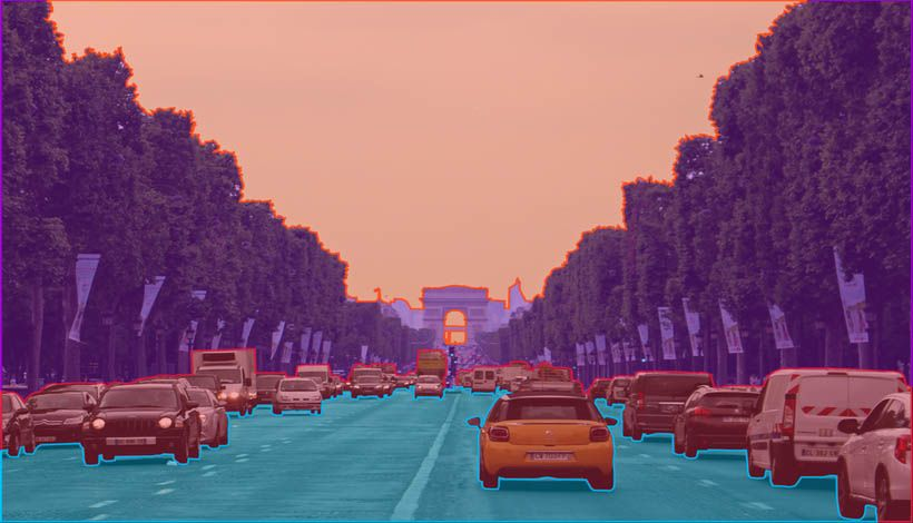
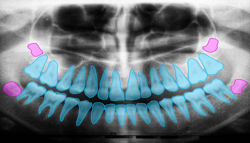
In this post, we will analyze a very similar area known as semantic image segmentation, a computer vision technique on the rise in fields such as medicine, automatic driving or satellite mapping.
Difference between image segmentation and object detection
At first glance, the two techniques may look very similar, but they are actually quite different.
Object detection attempts to detect the boundaries of objects by forming boxes and, in addition, it also attempts to identify those objects. On the other hand, semantic segmentation of an image consists of classifying all pixels in the image into one of the possible classes.
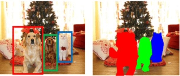
As can be seen in the image, a rectangular area has been found when detecting objects, while semantic segmentation has created a mask for their separation.
How does semantic image segmentation work?
There are many ways to perform semantic segmentation of an image, but most techniques follow a common pattern that consists of dividing the process into two stages known as encoding and decoding. In this post we are going to focus on the U-Net architecture, a model developed specifically for medical image segmentation.
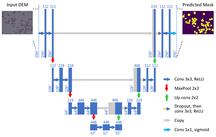
The first encoding stage is based on reducing the spatial dimensionality by means of pooling layers combined with convolutions. The aim of this process is to create an image feature map and reduce the number of network parameters.
The second decoding stage is completely symmetrical to the first one, increasing the dimensionality of the image to the original size by a combination of up-sampling and convolutions.
It should be noted that the layers of the encoding stage are giving their outputs to their respective layers of the decoding stage. The purpose of this is to maintain the context of the classification in order to reduce the amount of information lost by reducing the dimensionality of the image in the first stage.
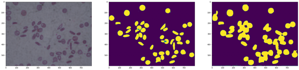
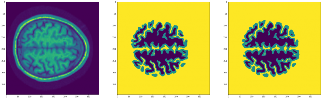
Results of a U-Net
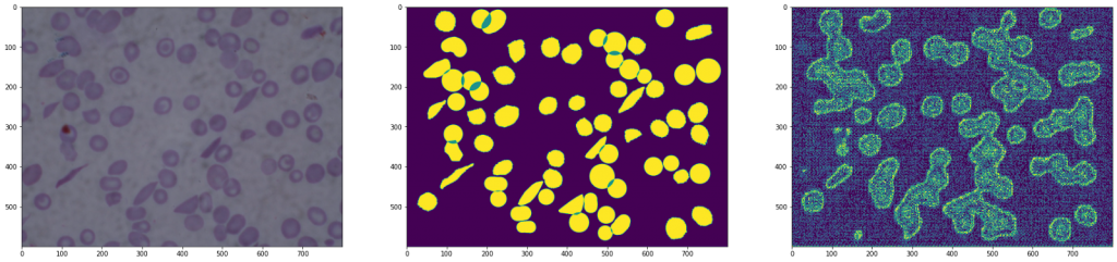
Result of an architecture without the copy of the results
As we can see in the images, the second architecture shows an image with a lot of noise, as information has been lost when downsampling followed by up-sampling.
Experimentation with PyTorch
Pytorch is a machine learning framework based on the Torch library. It is used in both computer vision and NLP (Natural language Processing) applications.
First we are going to download and load the dataset. This is a set of 394 x 394 MRI images.
url = 'https://mymldatasets.s3.eu-de.cloud-object-storage.appdomain.cloud/MRIs.zip'
wget.download(url)
with zipfile.ZipFile('MRIs.zip', 'r') as zip_ref:
   zip_ref.extractall('.')
path = Path('./MRIs')
imgs = [path/'MRIs'/i for i in os.listdir(path/'MRIs')]
ixs = [i.split('_')[-1] for i in os.listdir(path/'MRIs')]
masks = [path/'Segmentations'/f'segm_{ix}' for ix in ixs]
class Dataset(torch.utils.data.Dataset):
def __init__(self, X, y, n_classes=3):
self.X = X
self.y = y
self.n_classes = n_classes
def __len__(self):
return len(self.X)
def __getitem__(self, ix):
img = np.load(self.X[ix])
mask = np.load(self.y[ix])
img = torch.tensor(img).unsqueeze(0)
mask = (np.arange(self.n_classes) == mask[...,None]).astype(np.float32)
return img, torch.from_numpy(mask).permute(2,0,1)
dataset = {
'train': Dataset(imgs[:-100], masks[:-100]),
'test': Dataset(imgs[-100:], masks[-100:])
}
dataloader = {
'train': torch.utils.data.DataLoader(dataset['train'], batch_size=16, shuffle=True, pin_memory=True),
'test': torch.utils.data.DataLoader(dataset['test'], batch_size=32, pin_memory=True)
}
imgs, masks = next(iter(dataloader['train']))We are now going to implement the U-Net model. It is one of many possible variations on how to implement it, so we encourage you to write your own implementation.
def conv3x3_bn(ci, co):
return torch.nn.Sequential(
torch.nn.Conv2d(ci, co, 3, padding=1),
torch.nn.BatchNorm2d(co),
torch.nn.ReLU(inplace=True)
)
def encoder_conv(ci, co):
return torch.nn.Sequential(
torch.nn.MaxPool2d(2),
conv3x3_bn(ci, co),
conv3x3_bn(co, co),
)
class deconv(torch.nn.Module):
def __init__(self, ci, co):
super(deconv, self).__init__()
self.upsample = torch.nn.ConvTranspose2d(ci, co, 2, stride=2)
self.conv1 = conv3x3_bn(ci, co)
self.conv2 = conv3x3_bn(co, co)
def forward(self, x1, x2):
x1 = self.upsample(x1)
diffX = x2.size()[2] - x1.size()[2]
diffY = x2.size()[3] - x1.size()[3]
x1 = F.pad(x1, (diffX, 0, diffY, 0))
x = torch.cat([x2, x1], dim=1)
x = self.conv1(x)
x = self.conv2(x)
return x
class UNet(torch.nn.Module):
def __init__(self, n_classes=3, in_channels=1):
super().__init__()
c = [16, 32, 64, 128]
self.conv1 = torch.nn.Sequential(
conv3x3_bn(in_channels, c[0]),
conv3x3_bn(c[0], c[0]),
)
# Encoder
self.conv2 = encoder_conv(c[0], c[1])
self.conv3 = encoder_conv(c[1], c[2])
self.conv4 = encoder_conv(c[2], c[3])
# Decoder
self.deconv1 = deconv(c[3],c[2])
self.deconv2 = deconv(c[2],c[1])
self.deconv3 = deconv(c[1],c[0])
self.out = torch.nn.Conv2d(c[0], n_classes, 3, padding=1)
def forward(self, x):
# Encoder
x1 = self.conv1(x)
x2 = self.conv2(x1)
x3 = self.conv3(x2)
x = self.conv4(x3)
# Decoder
x = self.deconv1(x, x3)
x = self.deconv2(x, x2)
x = self.deconv3(x, x1)
x = self.out(x)
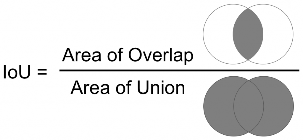
return xFinally, for training the model, we will use the IoU (Intersection over Union), which is the ratio between the area of overlap and the area of union between the two masks (the predicted and the ground truth).
And we have implemented the following fit function to perform the training:
device = "cuda" if torch.cuda.is_available() else "cpu"

def fit(model, dataloader, epochs=100, lr=3e-4):
   optimizer = torch.optim.Adam(model.parameters(), lr=lr)
   criterion = torch.nn.BCEWithLogitsLoss()
   model.to(device)
   hist = {'loss': [], 'iou': [], 'test_loss': [], 'test_iou': []}
   for epoch in range(1, epochs+1):
     bar = tqdm(dataloader['train'])
     train_loss, train_iou = [], []
     model.train()
     for imgs, masks in bar:
       imgs, masks = imgs.to(device), masks.to(device)
       optimizer.zero_grad()
       y_hat = model(imgs)
       loss = criterion(y_hat, masks)
       loss.backward()
       optimizer.step()
       ious = iou(y_hat, masks)
       train_loss.append(loss.item())
       train_iou.append(ious)
       bar.set_description(f"loss {np.mean(train_loss):.5f} iou {np.mean(train_iou):.5f}")
     hist['loss'].append(np.mean(train_loss))
     hist['iou'].append(np.mean(train_iou))
     bar = tqdm(dataloader['test'])
     test_loss, test_iou = [], []
     model.eval()
     with torch.no_grad():
       for imgs, masks in bar:
         imgs, masks = imgs.to(device), masks.to(device)
         y_hat = model(imgs)
         loss = criterion(y_hat, masks)
         ious = iou(y_hat, masks)
         test_loss.append(loss.item())
         test_iou.append(ious)
         bar.set_description(f"test_loss {np.mean(test_loss):.5f} test_iou {np.mean(test_iou):.5f}")
     hist['test_loss'].append(np.mean(test_loss))
     hist['test_iou'].append(np.mean(test_iou))
     print(f"\nEpoch {epoch}/{epochs} loss {np.mean(train_loss):.5f} iou {np.mean(train_iou):.5f} test_loss {np.mean(test_loss):.5f} test_iou {np.mean(test_iou):.5f}")
   return hist
model = UNet()
hist = fit(model, dataloader, epochs=30)After training the model, we can see the following result:
As we can see, it has worked very well.
Conclusion
Semantic image segmentation is a very useful and interesting field of computer vision, whose uses can bring great benefits in very different fields of research and development.
In this post we have focused on U-Net due to its excellent performance, but it is worth mentioning the wide variety of models such as FCN, SegNet and DeepLab that are also perfectly valid.
If you found this article interesting, we encourage you to visit the Algorithms category to see other posts similar to this one and to share it on social networks. See you soon!
