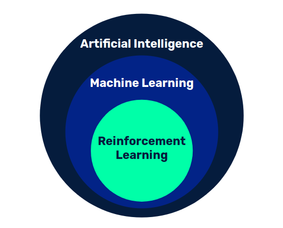
Although there is no consensus on the definition of artificial intelligence, we can say that it is the set of techniques whereby a computer system can exhibit intelligent behavior.
There are many approaches, such as expert systems, where rules are defined based on existing knowledge of a subject and are triggered according to the fulfillment of certain conditions. On the other hand, the branch of Machine Learning seeks to achieve such intelligent behavior through a learning process.
Usually we talk a lot about supervised learning, where the model is fed with data inputs and their corresponding desired outputs. After a period of training, the model learns the patterns that relate the inputs to the outputs, and is able to generalize by working successfully with new inputs that have not been seen previously.
On the contrary, there are models where learning takes place without any desired outputs, simply from the data itself. This is unsupervised learning, where we can find Clustering techniques or generative models.
However, there is a third variant, reinforcement learning, where this happens through the interaction between an agent and an environment. In this post we will study Q-learning, an ideal reinforcement learning technique to get into this field.
Markov decision processes
As mentioned above, the basis of this type of techniques is the interaction of the agent with the environment, which in general can be seen as a Markov decision process, where with each action performed by the agent, the state of the environment is updated and a reward is provided, which will be a numerical value that the agent will seek to maximize. This flow is shown below, taking as an example the video game Ms Pacman:
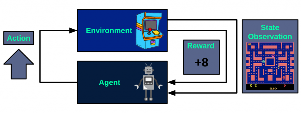
At each instant, the agent takes one of the available actions, in this case, move up. After performing this action, the environment will return the observation of the resulting state, that is, the next image of the game screen. In addition to this, a reward will also be returned, which will be +8.
Starting from this framework, the objective of reinforcement learning will be that the agent learns a policy that maximizes the rewards obtained, considering the policy as the function that for a state, returns the action to be performed.
Value function
If in each state we could know the cumulative reward that could be obtained by performing each of the available actions, it is clear that the policy we would follow would be to take the action that allows us to access a higher cumulative reward.
In Q-learning, we call Q to the value function that returns the expected cumulative reward of performing an action in a state, serving as a measure of the quality of that pair (state, action). Starting from this function, the policy to follow will be to take at each instant the action with the highest value according to our Q function.
In its tabular version, Q will be a table with as many rows as possible states and as many columns as available actions, where each element will be the approximation of the value for the corresponding pair (state, action).
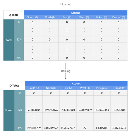
Once the table is initialized, the values will be updated iteratively in the following way

We see how the new value preserves part of the original and is updated with the new information: the reward obtained and the value of the best pair (state, action) for the state st+1 reached. The parameter α is a learning coefficient, which determines how much the old value is modified by the new information. On the other hand, γ it is a time preference factor that defines how much future rewards are valued over current ones.
The exploration-exploitation dilemma
If when we are learning the values of the Q function we act voraciously selecting the action with the best expected return, we are likely to fall into a local optimum, because we are not experimenting with other variants that may not be as good in the short term but may be better in the long term. On the contrary, if we do not focus on the good ones that we find, we will not get closer to better solutions. For this reason it is important to make a good balance between exploring new paths and exploiting the ones we already know are good.
A simple way to obtain this balance is to use Epsilon-Greedy. For each instant, with probability ∈, a random action will be taken (Exploration) and, in the opposite case, the action with the highest expected return will be taken (Exploitation). Depending on the value defined for ∈, more weight will be given to exploration or exploitation. Usually, a smart strategy is to vary this parameter throughout the training, so that at the beginning more weight is given to exploration, and progressively it is reduced in order to fine-tune the best solutions.
Conclusion
The technique we have seen, tabular Q-learning, is very interesting to introduce in this field. However, it has many limitations. On the one hand, if the environment is relatively complex, having a table with all combinations of states and actions is unmanageable. In addition, this approach is not able to work directly with continuous state and action spaces.
In future posts we will see Deep Q-Network, a variant of Q-learning where the table is replaced by a neural network, thus mitigating the limitations of the tabular version.
If you liked this post, we encourage you to visit the Algorithms category to see other articles similar to this one and to share it on social networks. See you soon!
