

The post Process Discovery: Methods and a Practical Example already explored this popular technique for deriving a process model from logs of the original system.
However, there is much more that can be done with those process logs. For example, we can combine what was done previously and evaluate it against reality. Or we can even generate the model ourselves, either using expert knowledge or by following specific steps to do so.
What is Process Conformance?
To verify how well a model aligns with reality, there is a discipline known as Process Conformance. This field focuses on obtaining various metrics that allow us to evaluate whether or not the model is appropriate.
Practical example of Process Conformance
Next, we’ll walk through a practical example to understand how this concept works. For this purpose, the example model we’ll use for process conformance testing is a representation of a payment system.
In this system, the customer begins by placing an order; next, their credit is checked, and the payment risk is assessed. The order is then evaluated, approved, or rejected, and finally, the customer is notified of the decision.
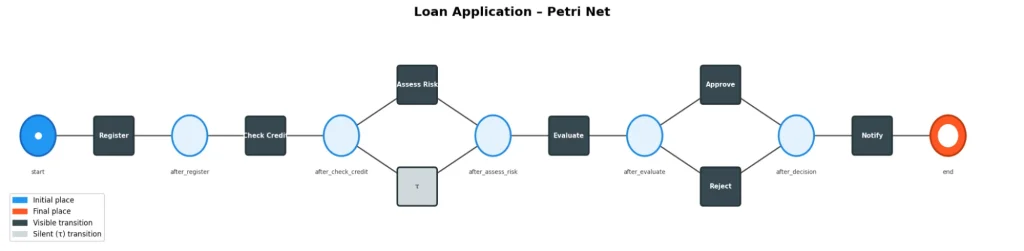
To evaluate the model, we generated 26 different traces. Each of these also belongs to one of the following 6 categories:
- Fully compliant with the model, including Assess Risk.
- Compliant with the model but without Assess Risk.
- One or more activities have been skipped.
- Out-of-sequence activities.
- Extra activities.
- Ends before reaching the last task (incomplete).
Next, we will evaluate the traces using two different methodologies: Token Replay and Alignment. Both techniques allow us to determine how closely our model matches the observed reality, but they use different approaches.
Token Replay methodology
First, we will use Token Replay to evaluate the model against the traces. This technique is the most obvious way to assess a model and, essentially, simulates how the observed trace would move through the generated model.
We start with a trace and replicate it in the model we have generated. For example:
Initial state:
Trace: Register -> Check Credit -> Assess Risk -> Evaluate -> Approve -> Notify
Tokens produced: None
Step 1.
Start of evaluation; the trace begins with “Register”; we create “Register”.
Trace: Register -> Check Credit -> Assess Risk -> Evaluate -> Approve -> Notify
Tokens produced: 1
Step 2.
The model consumes “Register” and produces “Check Credit”.
Tokens produced: 2
Tokens consumed: 1
Trace: Check Credit -> Assess Risk -> Evaluate -> Approve -> Notify
Step 3.
The model consumes “Check Credit” and produces “Assess Risk”.
Tokens produced: 3
Tokens consumed: 2
Trace: Assess Risk -> Evaluate -> Approve -> Notify
Step 4.
The model consumes “Assess Risk” and produces “Evaluate”.
Tokens produced: 4
Tokens consumed: 3
Trace: Evaluate -> Approve -> Notify
Step 5.
The model consumes “Evaluate” and produces “Approve”.
Tokens produced: 5
Tokens consumed: 4
Trace: Approve -> Notify
Step 6.
The model consumes “Approve” and produces “Notify”.
Tokens produced: 6
Tokens consumed: 5
Trace: Notify
Step 7.
The model consumes “Notify” and produces no events.
Tokens produced: 7
Tokens consumed: 6
Trace: None
At the end of the replay of this perfect trace, we have produced 7 tokens and consumed 6. Therefore, we did not run short of any tokens, nor were there any tokens left over in the trace.
Calculating the model’s fitness
The model’s fitness is equal to 0.5*(1 – (missing tokens / consumed tokens)) + 0.5*(1 – (remaining tokens / produced tokens)). In this case, the fitness is 1 since there are no missing or remaining tokens. In other words, the model perfectly describes the behavior observed in the trace.
However, if the trace does not behave exactly as the model expects, we have the following:
Initial state:
Trace: Register -> Check Credit -> Assess Risk -> Evaluate -> Alarm -> Approve -> Register -> Notify
Tokens produced: None
Step 1.
Start of evaluation; the trace begins with “Register”; we create “Register”.
Trace: Register -> Check Credit -> Assess Risk -> Evaluate -> Alarm -> Approve -> Register -> Notify
Tokens produced: 1
Step 2.
The model consumes “Register” and produces “Check Credit.”
Tokens produced: 2
Tokens consumed: 1
Trace: Check Credit -> Assess Risk -> Evaluate -> Alarm -> Approve -> Register -> Notify
Step 3.
The model consumes “Check Credit” and produces “Assess Risk”.
Tokens produced: 3
Tokens consumed: 2
Trace: Assess Risk -> Evaluate -> Alarm -> Approve -> Register -> Notify
Step 4.
The model consumes “Assess Risk” and produces “Evaluate”.
Tokens produced: 4
Tokens consumed: 3
Trace: Evaluate -> Alarm -> Approve -> Register -> Notify
Step 5.
The model consumes “Evaluate” and produces “Approve”.
The model is unable to consume “Alarm”; one token is missing from the model.
Tokens produced: 5
Tokens consumed: 4
Missing tokens: 1
Trace: Approve -> Register -> Notify
Step 6.
The model consumes “Approve” and produces “Notify”.
Tokens produced: 6
Tokens consumed: 5
Missing tokens: 1
Trace: Register
Step 7.
The model consumes “Notify” and produces no events.
The second “Register” was never consumed; one token remains.
Tokens produced: 7
Tokens consumed: 6
Missing tokens: 1
Remaining tokens: 1
Trace: Register
Now, the model’s fitness with respect to this trace would be 0.5*(1-1/6)+0.5(1-1/7) = 0.845.
Looking at the fitness, we can see how the model almost captures the behavior, but not completely. This is to be expected, since we intentionally created a trace that is not described by the model.
Applying this method to the traces we generated, we find that:
| Category | Fitness Media |
| Fully Approved | 1 |
| In accordance with Assess Risk | 1 |
| Extra activity | 0.97 |
| Incorrect order | 0.85 |
| Skipped activity | 0.82 |
| Incomplete | 0.77 |
The traces we intentionally generate by perfectly following the model have perfect fitness, while different defects have varying effects on fitness.
However, there is a fundamental limitation to using Token Replay. If events are recorded out of order or are missing, the effects on their fitness are very significant. This is because they cannot be consumed exactly as described by the model. However, it may well be that the only difference is a slight misalignment—a single event occurring before another, caused, for example, by inaccuracies in event logging. To account for these cases, we use the alignment metric.
Evaluation using Alignment
The alignment methodology for a model, unlike Token Replay, frames the problem as an optimisation problem, where we have the trace and its “equivalent” trace in the model. Alignment is, therefore, the minimum cost required to transform our trace into its equivalent according to the model.
To do this, there are three types of moves required when evaluating a trace using alignment: Move on Log, Move on Model, and Synchronous Move.
- Move on log. The event exists in the trace, but the model does not include such an event.
- Move on model. An event was expected by the model, but was not observed in the trace.
- Synchronous Move. The event in the trace matches its specification in the model.
Example of evaluation with Alignment
For example, for the trace:
Register → Assess Risk → Evaluate → Alarm → Approve → Register → Notify
| Trace | Model | Movement | Cost |
| Register | Register | Synchronous move | 0 |
| – | Check Credit | Move on model | 1 |
| Assess Risk | Assess Risk | Synchronous move | 0 |
| Evaluate | Evaluate | Synchronous move | 0 |
| Alarm | – | Move on log | 1 |
| Approve | Approve | Synchronous move | 0 |
| Register | – | Move on log | 1 |
| Notify | Notify | Synchronous move | 0 |
The total alignment cost is therefore 3, since we have 2 Move on Log and 1 Move on Model.
Applying this to our traces:
| Category | Average Total Alignment Cost | Move on log media | Move on model media |
| Fully Approved | 0 | 0 | 0 |
| In accordance with Assess Risk | 0 | 0 | 0 |
| Extra activity | 1 | 1 | 0 |
| Skipped activity | 1 | 0 | 1 |
| Incorrect order | 2 | 1 | 1 |
| Incomplete | 2 | 0 | 2 |
We can see that it is easier to diagnose errors. Errors such as incompleteness or incorrect task order are not as prevalent as in Token Replay, even though they remain significant.
The limitation of alignment-based conformance analysis is that it is considerably more computationally expensive. Thus, for sufficiently large traces, this type of analysis becomes difficult. For this reason, Token Replay may be preferred, especially since it is less robust to errors.
Conclusion
Conformance analysis allows us to evaluate, in a standardised way, how traces differ from a previously defined model. To this end, we have discussed two popular methods: Token Replay and Alignment.
We have also demonstrated how Token Replay works, provided examples, and shown how different errors affect the results. We have done the same with process alignment, finding that it is more accurate at diagnosing errors but is also computationally more expensive.
If you found this article interesting, we encourage you to visit the Data Science category to see other posts similar to this one and visit the Damavis website to learn about our projects. See you soon!
