What is Linear Programming?
The concept of Linear Programming or Linear Optimisation refers to that branch of mathematics that is dedicated to optimising (maximising or minimising) a linear objective function subject to constraints in the form of equations and/or inequalities.
Although it is an advanced branch of mathematics, its use is widespread in everyday life. For example, in managing monthly shopping by trying to spend as little money as possible while meeting a series of requirements.
In this post, we will define the basic concepts of Linear Programming and the different types that exist. In addition, we will introduce the Simplex method, a widely used algorithm to solve linear optimisation problems.
Basic fundamentals of Linear Programming
As the name indicates, in linear programming functions and constraints are linear. Therefore, the objective function is a linear function of n variables and the constraints must be linear equations or inequalities.
Definition of the optimisation problem
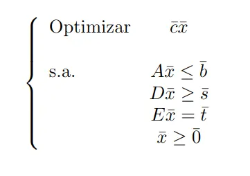
A general definition of a linear programming optimisation problem is:
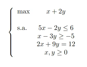
What do we really want to obtain as a solution? The solution is an n-dimensional vector in which all the constraints of the problem are satisfied and optimizes the objective function. There can be many vectors that meet the constraints and we call them feasible solution. Let’s see an example to illustrate more clearly the two concepts:
The region of feasible solutions in this case would be
{}.
As we can see, the constraints that appear can be of type inequality and equality, but to use the Simplex algorithm we need the constraints to be all of equality (although the implementation that we will see later is flexible and does not require such a condition), in addition to other conditions that we will mention shortly.
Standard Linear Programming optimisation problem
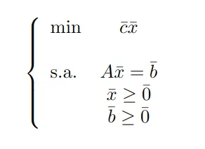
For this, we are going to introduce another way of expressing an optimisation problem and that is the Standard Form of a Linear Programming Optimisation Problem:
The objective is to be able to transform any type of optimization problem to its standard form. To do this we need a way to perform this transformation and the methodology that allows this consists of the following steps:
- If the problem is to maximise the objective function 𝑐̄x̄, we must change to minimise -𝑐̄x̄.
- If there is any independent term of the negative equality constraints, we change the sign to the entire constraint.
- Inequality constraints can be converted into equality constraints by introducing so-called slackvariables:
- If we have ai1x1 +...+ ainxn <= bi, we can transform it using a variable xhi >= 0 thus: ai1x1 +...+ ainxn + xhi = bi.
- If we have ai1x1 +...+ ainxn >= bi, we can transform it using a variable xhi >=0 thus: ai1x1 +...+ ainxn - xhi = bi.
- If any decision variable xi does not meet the non-negativity condition is not satisfied, then we replace it by 2 new variables yi, zi such that xi = yi + zi.
Let’s see an example of how to pass an optimization problem to its standard form:
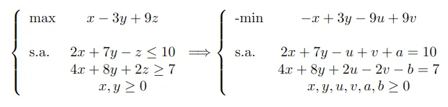
Fundamentals of the Simplex Method or Algorithm
We will consider only problems in their standard form for the Simplex method. For this, there is an important concept which is basic feasible solution.
What is the Basic Feasible Solution
Let us consider an optimization problem in its standard form. Let us fix some concepts that are necessary to define a basic feasible solution, where A is the matrix of coefficients of equality constraints of dimension mxn:
- Basic Matrix: A square (same number of rows and columns) non-singular (its inverse exists) submatrix B of dimension m of A is called a basic matrix. Moreover, B is a feasible basis matrix if B-1b̅ >=0.
- We will call N the submatrix of A with dimension mx(n-m) that has as columns the columns of A that are not in B.
- Let x̄B be the vector of decision variables associated with the columns of the matrix A necessary to construct B. They are called basic variables.
- Let x̄N be the vector of decision variables associated to the columns of matrix A necessary to construct N. They are called non-basic variables.
- If we require that x̄N = 0̄ we would have:
Ax̄ = b̅Bx̄B + Nx̄N = b̅ Bx̄B + N0̄ = b̅ Bx̄B = b̅ x̄B = B-1b̅
Considering the above, the solution x̄ = (B-1b̅, 0̄) of the system of equations Ax̄ = b̅ is called the basic feasible solution if B-1b̅ >= 0.
Simplex Method or Algorithm procedure
Let us first fix the notation necessary to explain the procedure.
- Consider B a nonsingular square submatrix of dimension m of A. Then we denote by I and J the sets with the indices associated to the columns of B and N, respectively.
- Consider and āj to be the j-th column of A, we denote the vector B-1āj for ȳj.
- Consider and 𝑐̄B as the vector formed by the coefficients of the objective function associated to the columns of the submatrix B, we denote by zj the value 𝑐̄Bȳj = 𝑐̄BB-1āj.
The Simplex method searches all the basic feasible solutions one by one and verifies whether they are optimal or not. It does this iteratively until it finds the optimal basic feasible solution or until it verifies that the problem has no solution.
Suppose that x̄B is a basic feasible solution, then the following steps are performed:
- If there exists such that zj - cj > 0 and ȳj < = 0̄, then the optimisation problem in its standard form does not admit an optimal solution.
- If zj - cj <= 0, ∀j ∈ J, then x̄ = (B-1b̅, 0̄)is an optimal feasible solution ↔ zj - cj <= 0, ∀j ∈ J. If it is satisfied that max{zj - cj: j ∈ J} = 0, then the problem is feasible but the optimal solution is not unique.
- If the Simplex has failed to determine any decision, a new basic feasible solution is computed and the above steps are reapplied.
Simplex method in Python with SciPy
Now that we have explained the ins and outs of the Simplex method, let’s see how to use it in Python. The optimize module of the SciPy library contains a method called linprog() for solving linear programming optimization problems (see the official documentation for more information). It is worth remembering that this method does not require all constraints to be equal, it also includes the option to incorporate least or equal constraints.
Consider the following optimization problem:
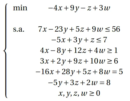
In total there are 6 constraints (2 of each type) and 4 decision variables, resulting their resolution by hand a very expensive process. The Python implementation is as follows:
from scipy.optimize import linprog
import numpy as np

A_ub = np.array([[7, -23, 5, 9], [-5, 3, 1, 0], [-4, 8, -12, -4], [-3, -2, -9, -10],
     [-1, 0, 0, 0], [0, -1, 0, 0], [0, 0, -1, 0], [0, 0, 0, -1]])
A_eq = np.array([[-16, 28, 5, 8], [0, -5, 3, 2]])
b_ub = np.array([56, 7, -1, -6, 0, 0, 0, 0])
b_eq = np.array([5, 8])
c = np.array([-4, 9, -1, 3])

linprog(c=c, A_ub=A_ub, b_ub=b_ub, A_eq=A_eq, b_eq=b_eq, method="simplex")
The result we get is:
       con: array([ 5.68434189e-13, -2.84217094e-14])
       fun: -60.305084745761874
message: 'Optimization terminated successfully.'
       nit: 9
    slack: array([5.68434189e-13, 2.19237288e+02, 7.02389831e+02,
               7.75508475e+02, 7.26101695e+01, 3.17457627e+01,
               5.55762712e+01, 0.00000000e+00])
    status: 0
    success: True
          x: array([72.61016949, 31.74576271, 55.57627119,  0.        ])
The method has successfully completed its search for the optimal feasible solution in 9 iterations. The optimal solution obtained is x̄ = (72.61, 31.75, 55.58, 0.0) and the minimum value of the objective function is -60.31.
Here is the end of today’s post. If you found it interesting, we encourage you to visit the Algorithms category to see all the related posts and to share it in networks with your contacts. See you soon!
