
In two previous posts we introduced the basic concepts of Fuzzy Logic and linear programming with the Simplex method. As promised, in this post we are going to join these two concepts and introduce fuzzy linear programming.
In many real-world cases, the data we have does not meet the accuracy requirements of linear programming implementation. In this sense, we need a more flexible methodology that includes adding uncertainty in the data, which is where fuzzy linear programming comes into play.
Bellman-Zadeh Method
We are going to define the fuzzy objective, constraint and decision and then introduce the Bellman-Zadeh decision making process. We define X as the set of all possible alternatives, containing the solution of the decision problem.
Fuzzy target: It is defined as the fuzzy set ![]()
![]() over X with membership function
over X with membership function ![]()
![]() .
.
Fuzzy Constraint: It is defined as the fuzzy set ![]()
![]() over X with membership function
over X with membership function ![]()
![]() .
.
Fuzzy Decision: It is defined as the fuzzy set ![]()
![]() over X with membership function
over X with membership function ![]()
![]() .
.
The Bellman-Zadeh method establishes as the optimal alternative ![]()
![]() that which maximizes the membership function of the fuzzy decision:
that which maximizes the membership function of the fuzzy decision:

In this way, the fuzzy decision solves the decision making problem, since for each alternative it establishes the degree to which the constraints and the objective are satisfied. The Bellman-Zadeh method provides an optimal alternative as ![]()
![]() . This decision making process is known as defuzzification.
. This decision making process is known as defuzzification.
The objective and the fuzzy constraint have equal weight on the fuzzy decision, neither has a more important role than the other. This is why the Bellman-Zadeh method is symmetric.
The membership function they proposed for the fuzzy decision is:

where ![]()
![]() . This definition of the fuzzy decision membership function is motivated because sometimes we are interested in a certain asymmetry in the way of compatibility between fuzzy constraints and fuzzy objectives.
. This definition of the fuzzy decision membership function is motivated because sometimes we are interested in a certain asymmetry in the way of compatibility between fuzzy constraints and fuzzy objectives.
Symmetric fuzzy linear programming
In many cases we do not want to optimize the objective function or strictly comply with the constraints. In these cases we want to reach (or not exceed) a certain level set as objective, in the same way that there is a certain degree of flexibility with respect to the constraints. For these cases we propose a variant of linear programming problems.
A formal definition of a symmetric fuzzy linear programming optimization problem is:
The symbol ![]()
![]() is a fuzzy version of the order relation
is a fuzzy version of the order relation ![]() and could be defined as “essentially smaller than or equal to”. Since for Bellman and Zadeh the fuzzy objectives and constraints are of equal importance, Zimmermann expressed the problem as follows, calling it Zimmermann’s Symmetric Fuzzy Linear Programming Optimization Problem:
and could be defined as “essentially smaller than or equal to”. Since for Bellman and Zadeh the fuzzy objectives and constraints are of equal importance, Zimmermann expressed the problem as follows, calling it Zimmermann’s Symmetric Fuzzy Linear Programming Optimization Problem:
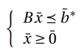
In order to connect fuzzy linear programming problems with classical linear programming problems, Zimmermann considered the membership functions of each constraint to be a trapezoidal fuzzy number on the right-hand side:
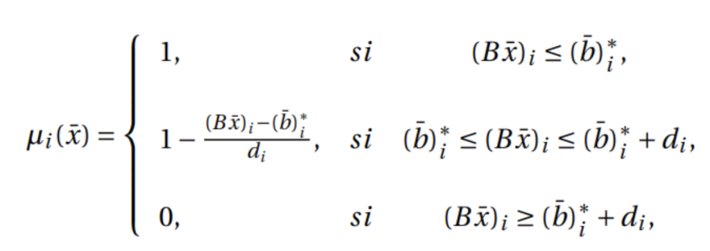
where ![]()
![]() is a constant that is chosen subjectively indicating the degree to which the i-th constraint can be exceeded;
is a constant that is chosen subjectively indicating the degree to which the i-th constraint can be exceeded; ![]() indicates the degree to which each
indicates the degree to which each ![]() satisfies the i-th constraint.
satisfies the i-th constraint.
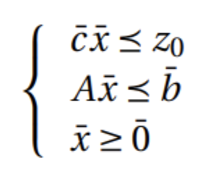
Recall that we want to solve the following problem: ![]()
![]() . If we add a new variable (img19) we can pose the problem as a classical linear programming problem:
. If we add a new variable (img19) we can pose the problem as a classical linear programming problem:
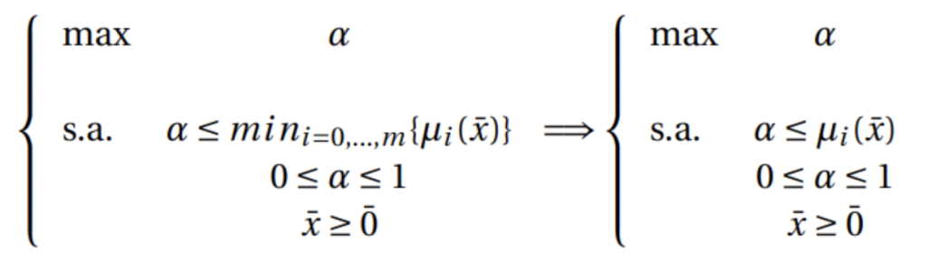
If we consider the membership function proposed by Zimmermann (trapezoidal on the right), we would have the following problem:
If ![]()
![]() is the optimal solution vector,
is the optimal solution vector, ![]() is the maximizing solution with membership degree
is the maximizing solution with membership degree ![]() .
.
Practical example
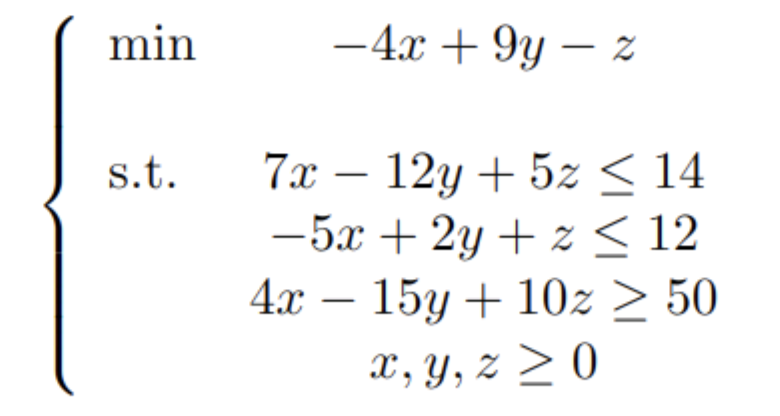
Let’s give an example of how we can deal with an optimization problem with non-exact data using fuzzy linear programming. To do so, let us first consider the following optimization problem:
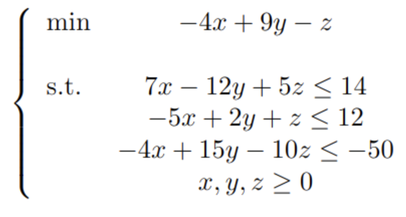
As we saw in the linear optimization post, we will change the constraints of the type ![]()
![]() by those of the type
by those of the type ![]() , simply altering the sign of the numbers, for convenience for the approach of the fuzzy problem:
, simply altering the sign of the numbers, for convenience for the approach of the fuzzy problem:
We solve the problem with Python:
from scipy.optimize import linprog
import numpy as np

A_ub = np.array([[7, -12, 5], [-5, 2, 1], [-4, 15, -10]])
b_ub = np.array([14, 12, -50])
c = np.array([-4, 9, -1])

linprog(c=c, A_ub=A_ub, b_ub=b_ub, method="simplex")
The result we obtain is:
message: Optimization terminated successfully.
 success: True
  status: 0
     fun: 18.205882352941185
       x: [ 1.029e+00  3.588e+00  9.971e+00]
     nit: 3
We see that the solution vector we obtain is ![]()
![]() with optimum value 18.21.
with optimum value 18.21.
We now pose the problem so that there is some flexibility in the constraints and the objective function. We fix that the optimum has to be at least 15, then the original problem would be as follows:

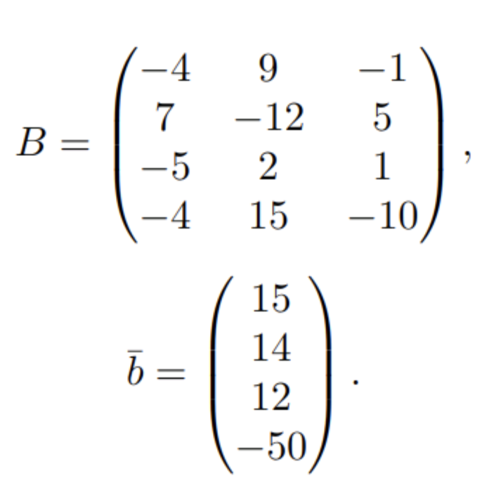
Following the nomenclature introduced by Zimmermann, we have:
In addition, the following ranges are established in which each specification can be transgressed:
Objective function: [15, 18,21].
Constraint 1: [14, 16]
Constraint 2: [12, 15]
Constraint 3: [-50, -48]
We obtain from these ranges the different ![]()
![]() :
:
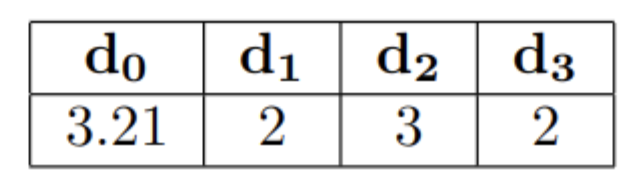
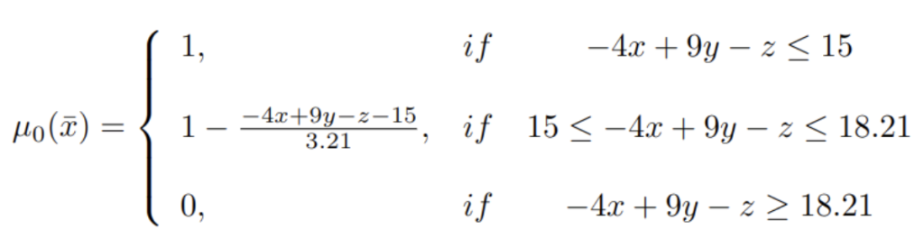
Each ![]()
![]() corresponds to the amplitude of each rank provided with respect to the problem specifications. Recall that the fuzzy sets modeling the problem specifications are trapezoidal on the right-hand side, we will illustrate the membership function for the first specification and the rest is drawn in the same way:
corresponds to the amplitude of each rank provided with respect to the problem specifications. Recall that the fuzzy sets modeling the problem specifications are trapezoidal on the right-hand side, we will illustrate the membership function for the first specification and the rest is drawn in the same way:
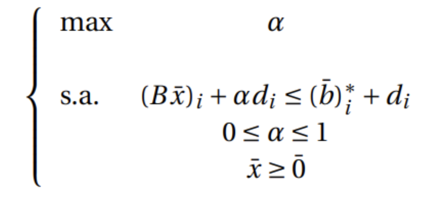
The classical linear programming problem associated with the original fuzzy problem is given by:
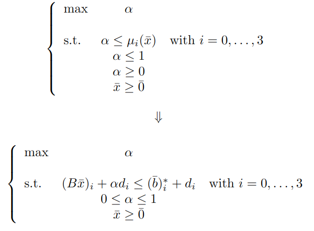
With the expressions of the 4 membership functions obtained and substituting them, we get the following:
We solve the problem with Python:
from scipy.optimize import linprog
import numpy as np

A_ub = np.array([[-4, 9, -1, 3.21], [7, -12, 5, 2], [-5, 2, 1, 3], [-4, 15, -10, 2], [0, 0, 0, 1]])
b_ub = np.array([18.21, 16, 15, -48, 1])
c = np.array([0, 0, 0, -1])

linprog(c=c, A_ub=A_ub, b_ub=b_ub, method="simplex")
We obtain the following result:
message: Optimization terminated successfully.
 success: True
  status: 0
     fun: -0.8734970521331415
       x: [ 5.662e-01  2.989e+00  9.232e+00  8.735e-01]
     nit: 5
We see that the solution vector we obtain is ![]()
![]() with an optimal value of 15.4, which is below the 18.21 we obtained with the classical linear optimization problem. The value of indicates that the problem admits solution with the new considerations with a degree of compatibility of all of them of 0.87.
with an optimal value of 15.4, which is below the 18.21 we obtained with the classical linear optimization problem. The value of indicates that the problem admits solution with the new considerations with a degree of compatibility of all of them of 0.87.
Conclusion
The aim of this post has been to unite fuzzy logic with classical linear programming, giving rise to fuzzy linear programming. The fact of making more flexible some requirements imposed by linear programming can give us better results, as we have seen with the practical example.
Bibliography
[1] Masatoshi Sakawa, Hitoshi Yano, Ichiro Nishizaki, and Ichiro Nishizaki. Linear and multiobjective programming with fuzzy stochastic extensions. Springer, 2013.
[2] Hans-Jürgen Zimmermann. Fuzzy set theory—and its applications. Springer Science & Business Media, 2011.
[3] Hans-Jürgen Zimmermann. Fuzzy sets, decision making, and expert systems, volume 10. Springer Science & Business Media, 2012.
So much for today’s post. If you found it interesting, we encourage you to share it in networks with your contacts, see you soon!
