In the post Natural Language Processing with Python the concept of NLP was introduced and an example of the use of the well-known GPT-3 text generation model was shown. In short, the system proposed by OpenAI is a generative artificial intelligence model capable of creating texts that emulate the writing ability of a human.
However, the field of natural language processing is not exclusive to generative models, and in areas such as computer vision we also find such models, but in this case capable of generating images instead of text.
In this post we will introduce one of these well-known generative models in computer vision: Generative Adversarial Networks (GAN).
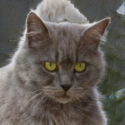
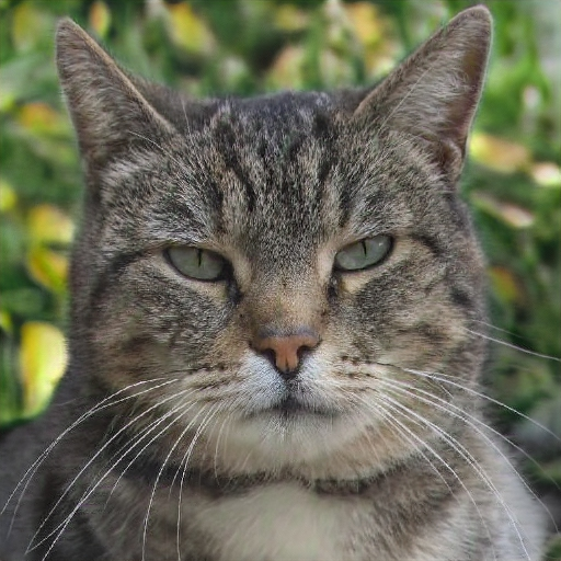
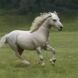
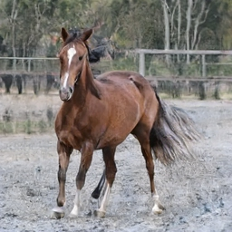
But before getting to know this kind of networks, if I propose you to identify which of the images you see below are real and which are not, you will probably find it difficult to make up your mind. You may even be surprised if I tell you that all of them have been artificially generated from a GAN.
Basic structure of a GAN
In 2014, a research group at the University of Montreal led by Dr Ian Goodfellow proposed a new framework for generative neural networks. First of all, the main goal of generative networks is based on trying to get a certain piece of data to adopt the distribution of another set of data. In other words, the aim is to make a given input so similar to the desired distribution that the generated data is indistinguishable from a real data from that distribution. In other words, if we are talking about images, to be able to generate an image that looks like the real thing.
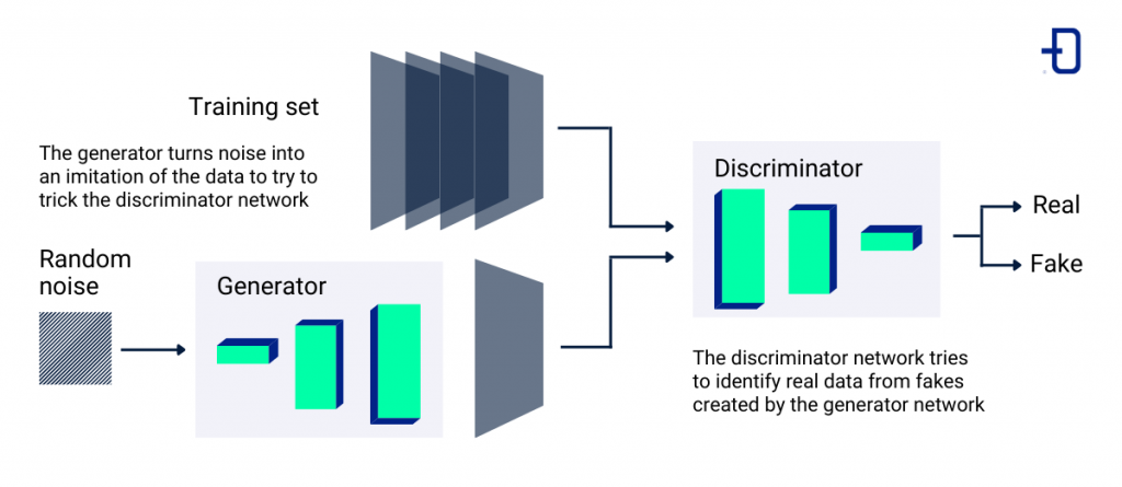
There are many solutions to achieve this goal. However, the proposed solution with generative adversarial networks is quite intuitive. It is mainly based on the use of 2 competing networks. On the one hand, we have a network called generator G and a different network called discriminator D.
The aim of the generator is to be able to capture the distribution of the data and from a series of random values generate an image that resembles in form and content the images of the data set being used. In contrast, the task of the discriminator will be to discern whether a given image corresponds to a real image or whether it has been generated by its antagonistic network, the generator.
If we look at this type of network from a mathematical point of view, we can see that it is a problem associated with game theory. Specifically, we consider a zero-sum game where the generator tries to minimise the same loss function that the discriminator will try to maximise.

Looking at the proposed loss function we can distinguish the following elements:
- D(x) is the discriminator’s estimate of the probability that a sample x belongs to the real data set.
- Ex is the expected value of membership that sample x has the same distribution as the real data over all real samples.
- G(z) is the output of the generator taking as input a set of random values (noise) denoted by z.
- D(G(z)) is the discriminator’s estimate of whether the output obtained by the generator is true or false.
- Ez is the expected value of the output obtained by the generator. In fact, it is the expected value over the distribution of all false samples, that is, created by the generator.
As can be seen, the formula is derived from the loss function widely used in Machine Learning known as Cross Entropy.
Training and common problems
After knowing the basic structure of this type of generative networks, we can introduce the usual training strategy. Since this type of network is actually composed of two independent networks, the training consists of training each of these networks together.
First, the generator will produce an image and this will be evaluated by the discriminator in the same iteration of the training. Therefore, the result of the discriminator will influence the weight update of the generator and by means of the backpropagation algorithm both networks will be updated. This will be repeated in each iteration of the training. Depending on the problem faced with this strategy, variations are applied, such as stopping training the discriminator at a certain point or not applying the weight update of the discriminator in all iterations.
Although GANs can generate good results, it is true that they do have some disadvantages. We can list three of them:
- Unstable convergence. Due to the competition between the two networks, the balance point is difficult to achieve. This causes the loss function during training to be very irregular and the results can vary a lot between periods.
- Mode collapse. This problem occurs when the generator is only able to generate a subset of images that adopt the distribution of the target data and for any given noise value generates the same output. The discriminator is unable to differentiate it from a real image, but in turn the results are all extremely similar.
- Gradient fading. Conversely, when the discriminator is able to distinguish too well between real and artificial data the weight update that occurs in the generator is very small. This results in the weights of the earliest layers not varying between epochs and therefore the network does not learn.
Although the original version of the GANs have these disadvantages, there are many variations that alleviate some of these problems.
Conclusion
In this post we have seen a brief theoretical introduction to another type of generative network. Usually this kind of networks are widely used in the field of computer vision because they fit very well with convolutional networks.
In fact, it is increasingly common to find uses of these networks in fashion, design or even digital recreations for video games. However, the ethical side should not be neglected, as these networks became famous after being used to create famous deepfakes.
In short, it is a type of neural architecture that is complex but with great potential. If you want to know more about this type of network and many others, be sure to visit the Damavis blog.
