Convolutional Neural Networks applied to Hungry Geese

Hungry Geese is a version of the mythical game “Snake”, but with geese, so that multiple agents compete against each other with the goal of surviving longer. This game was born in a Kaggle competition, developed between January 26, 2021 and August 10, 2021. In it, geese must not starve to death or impact opponents or themselves. One of the differences with the “Snake” game is that there are no limits along the edges of the board, so when the goose leaves from one of the 4 sides, it appears on the opposite side.

This article will explain how a basic artificial intelligence has been implemented with convolutional neural networks that is able to compete at a good level. It should be noted that this model will not be superior to another one implemented by Reinforcement Learning, but the results of the training performed can be seen more quickly.

Game rules

The objective is to survive as many turns as possible by feeding to stay alive and without colliding with your own goose or that of other agents. The rules of the game are as follows:

Four agents compete on an 11×7 cell board by indicating one of the following actions each turn: NORTH, SOUTH, EAST or WEST.
It is not allowed to make 180º turns, i.e. to return to the square occupied in the previous turn.
Each game consists of 200 episodes. The agent with the highest rating or the last surviving agent wins the game.
If an agent eats a piece of food, a segment is added to his body.
Every 40 episodes, the goose loses a segment, regardless of whether or not it has eaten previously.
Agents must make a movement decision in less than 1 second. If this is exceeded, the time difference is added to a counter. If this counter reaches 60 seconds, the agent is eliminated from the game.

Convolutional neural networks with supervised training

Convolutional neural networks with supervised training have been applied to create an artificial intelligence that can compete, above all, with other agents implemented with classical algorithms such as Minimax or Monte Carlo Tree Search (MCTS).

Supervised artificial intelligence models require a training dataset containing a “label” that indicates what the outcome should be given some variables. For this case, training datasets have been obtained from real games extracted by scraping the Kaggle metadata set.

Using this technique, more reliable datasets can be obtained by downloading the games of the best agents (those with scores above 1200, which have entered positions to obtain gold) because their actions are assumed to be the most correct. However, they are not perfect agents and they also lose games or make moves that are not optimal, so in the dataset there are also moves with actions that are not 100% valid and that the agent will learn wrongly.

It is worth mentioning that, in the competition, those who have achieved a score between 1050 and 1080 have obtained the bronze medal, those from 1080 to 1210 the silver medal and from 1210 onwards the gold medal, being 1312 the score obtained by the winner.

In the case of the Hungry Geese game, the variables are the current state of the board, that is, the positions occupied by the bodies of each agent, the positions occupied by food, or any other data that gives information about the board. The “label” is the action (NORTH, SOUTH, EAST or WEST) that should be performed given a board state.

Hungry Geese is a game in which all players must move at the same time, unlike other games where each player has a turn to decide a move.

This means that each player must decide at the same time what is the best action to take without knowing what action the opponent will take at the same time. This makes it possible to save up to 4 board states with their respective labels in the same turn, i.e. one for each player, so that larger data sets can be created in fewer games and, therefore, in less time.

From the real games extracted, the current board state and the move made by each agent has been saved so that, at the time of encoding the input for the neural network, there are four different views and four different decisions for the same state, that is, one for each agent.

Neural network input and output

Once the training data set has been obtained, it is necessary to encode the variables and actions to a valid structure for neural networks. Recall that the input data to the neural network contains the current state of the board, which has been encoded in a binary matrix of size (11, 7, 17), that is, 11 columns, 7 rows and 17 channels. This means that each cell of the board of size 11 x 7 is represented by 17 binary variables. Each channel of the matrix encodes a different piece of information on the board.

The value in the matrix, for all its channels, is 1 if the position on the board corresponds to the matrix cell to be represented in the channel. The value is 0 if nothing is to be represented at that position in the matrix. If an agent is dead, the channels representing the current position on the board will have all their cells with the value 0.

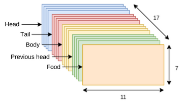
The first four channels encode the head positions of each agent, with one channel per agent. Each channel is one-hot since there is at most one value that is not 0.
Channels 5 through 8 indicate the tail position of each agent. Each channel is one-hot.
Channels 9 to 12 encode the positions of the whole bodies of each agent. These channels are not one-hot.
Channels 13 through 16 indicate the positions that the agents’ heads occupied in the previous board state. Each cell is one-hot.
Channel 17 indicates all the positions occupied by the food, and there may be one or two pieces of food at a time.

With this type of coding, the model can infer the length and shape of the agent from the position of the head, body and tail. In addition, the direction it has taken with respect to the last head position and the position of the other agents to avoid collisions.

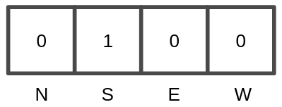
The output of the neural network is a 1×4 matrix with the probabilities of performing each of the 4 possible actions that the game has (NORTH, SOUTH, EAST or WEST). The action with the highest probability is the one that is finally performed given the current state of the board in each turn.

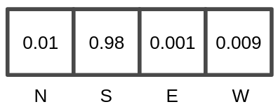
For the training phase, a 1×4 one-hot matrix is used with the action performed during the acquisition of the dataset given a board state.

Neural network architecture

The implemented neural network consists of a first block, called convolutional block, which is repeated 6 times, followed by a Global Average Pooling layer [3], to minimize the possibility of overfitting by reducing the number of parameters in the model, and ending with two layers of fully connected neurons of 1024 and 512 neurons, respectively, whose activation function is Leaky ReLU. The output layer consists of 4 neurons, which are the four possible actions that can be performed by the agent. The complete architecture of the neural network can be seen in the following figure.

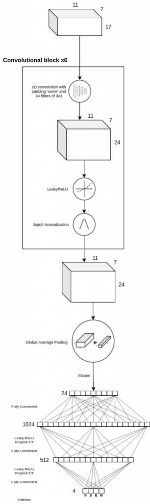
The convolutional block consists of a two-dimensional convolutional layer, with an automatic padding that allows the input and output of this layer to be equal in height and width, and 24 3×3 filters.

As explained above, the size of the model input is (11, 7, 17), so by applying automatic padding and 24 3×3 filters, the output of the convolutional layer will be (11, 7, 24). Next, the Leaky ReLU trigger function is applied. Finally, a Batch Normalization layer is used to standardize the output of the convolutional layer to the input of the next layer, transforming the values to mean 0 and standard deviation 1. Batch Normalization allows using a higher learning rate without a risk of divergence, as well as regularizing the model and reducing the need to use Dropout [1, 2]. This same block is repeated 6 more times, obtaining a final output of size (11, 7, 24).

Finally, two hidden layers of fully connected neurons are applied, of 1024 and 512 neurons, respectively, with a Leaky ReLU activation function and a Dropout of 0.5.

Training

The optimizer used in the model is Stochastic Gradient Descent with Momentum (SGDM) [4, 5], having to adjust the learning rate and momentum parameters. The training starts with a fixed learning rate at 0.01 that decreases by a constant factor of 0.3 when there is no improvement in the model in a given number of epochs, down to a minimum of 0.0001, while the momentum parameter is kept constant throughout the training at 0.9 [6].

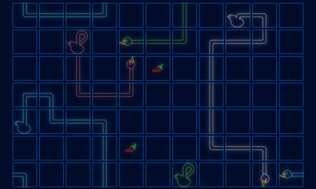
In 10 epochs an accuracy of 0.75 has been reached in the validation data set, that is, in the records that have been used neither for training nor for testing. In 13 epochs an accuracy of 0.8102 was obtained, with no improvement in the next 25 epochs, so training was stopped. The final result in a real game in which the 4 geese use the same trained convolutional neural network is as follows:

As can be seen, the model has been able to infer that the goose must avoid contact with itself and its rivals, that it must go for the food in order not to die and win, and even protect itself. From step 95 onwards it is possible to see that the blue goose turns around itself as the best option to avoid colliding with the rivals around it. On the other hand, from step 104 onwards you can see that the white goose does not take the food next to it because it knows that it will end up in an enclosed space from which it will not be able to get out.

I hope you liked this article which explains how you can easily implement a basic artificial intelligence with convolutional neural networks that is able to compete and with which you can see immediate results of the training performed. The repository in which this neural network has been implemented, as well as other implementations, can be found here.

If you want to know more about neural networks, I advise you to read the following articles by other Damavis members:

Bibliography

[1] Nitish Srivastava, Geoffrey Hinton, Alex Krizhevsky, Ilya Sutskever and Ruslan Salakhutdinov. Dropout: A simple way to prevent neural networks from overfitting. Journal of Machine Learning Research, 15(56): 1929–1958, 2014.

[2] Sergey Ioffe and Christian Szegedy. Batch normalization: Accelerating deep network training by reducing internal covariate shift. CoRR, abs/1502.03167, 2015.

[3] Min Lin, Qiang Chen and Shuicheng Yan. Network in network. In 2nd International Conference on Learning Representations, Conference Track Proceedings, Banff, AB, Canada, 2014.

[4] B.T. Polyak. Some methods of speeding up the convergence of iteration methods. USSR Computational Mathematics and Mathematical Physics, 4(5):1–17, 1964

[5] Nicolas Loizou and Peter Richtárik. Momentum and stochastic momentum for stochastic gradient, newton, proximal point and subspace descent methods. Computational Optimization and Applications, 77, 12 2020.

[6] Kaiming He, Xiangyu Zhang, Shaoqing Ren and Jian Sun. Deep residual learning for image recognition. CoRR, abs/1512.03385, 2015.

Convolutional Neural Networks applied to the game Hungry Geese