The kernel trick is a typical method in machine learning to transform data from an original space to an arbitrary Hilbert space, usually of higher dimensions, where they are more easily separable (ideally, linearly separable). This technique is the basis of Support Vector Machines, since these, without kernels, can only properly separate spaces that are linearly separable, but with the kernel trick they can operate with virtually any space, even if it is not Euclidean, such as molecules or graphs of friends in a social network.
In this post we want to not only show the concept behind the kernel trick, but also give an example in a non-Euclidean space to visually demonstrate the effect of kernelizing data.
Kernel Trick: Theoretical basis
To understand kernelization we must first understand what a Hilbert space is. A Hilbert space is defined as an inner product space that is complete with respect to the norm vector defined by the inner product, and while all properties are important, they are beyond the scope of this post, so we will focus on it having a definite inner product. This space is more permissive than a Euclidean one and, moreover, is where the data works once kernelized.
Next, we need to understand what a kernel is. A kernel is a function that receives two points and returns a value, with the added properties that the function is symmetric, such that f(x,v)=f(v,x), and that it is a positive semidefinite function. If these properties are satisfied, when we apply the kernel function, we are applying the equivalent of an inner product on an arbitrary Hilbert space corresponding to that kernel, in many cases an unknown space but one that we know exists.
In short, when we apply a kernel on the data, we are lifting it into a Hilbert space, in some cases, of infinite dimensions. But with this alone we still do not have the full power of kernelization: it is necessary that the method we are applying is also kernelizable and, for that, we simply have to keep in mind that whenever points are used, they are only used to compute inner products, so that the inner product function can be replaced by the kernel function.
Once this change is applied, we are operating in the arbitrary Hilbert space, instead of the original space. This is what we refer to as the “kernel trick” and allows us to raise the data to very interesting spaces, some of them having infinite dimensions.
Case study
All the code to obtain the results shown in this section, and even additional 3D visualizations of the data, is available in the Damavis repository. The 3D visualizations require running the notebook locally.
To demonstrate the space transformation and the power of kernelization, we will proceed to classify molecular data, where each point represents a molecule, and operate on it with SVMs and visualize it with kernel-PCA.
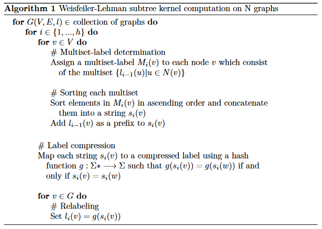
First we have to define a kernel that can operate on graphs. In our case, we define the Weisfeiler-Lehman kernel, which is based on a graph isomorphism test. Once the kernel is defined, we have to apply the kernel on the data. To explain the kernel, we use pseudo-code, where G(V,E,l) is a graph defined by its nodes (V), its edges (E) and the node labels (l). Once the multisets of nodes of each graph have been computed, we simply obtain the intersection of elements between the graphs and return the number of elements in common.
The data is the MUTAG dataset, consisting of 188 graphs, with 17.93 mean nodes per graph, 2.2 edges per mean node, 125 graphs belonging to class 1, and 63 to class -1. A small but well-known dataset for benchmarking algorithms on molecular graphs.
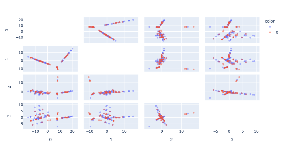
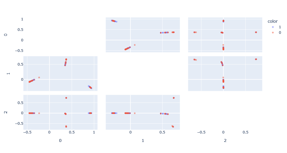
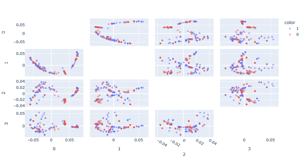
We apply the kernel function on the data to obtain the kernel function matrix and apply kernel-PCA on this matrix to obtain a representation of this space. What is interesting is that we can see how in the principal dimensions there are patterns that we would not have been able to see in its graph form.
However, there is the problem that, compared to a classical PCA, there is no concept of explained variance because the Hilbert space in which the PCA is made is unknown. Moreover, the space has as many dimensions as points, so it is interesting for visualization, but not very useful for classification.
Another interesting property of kernels is that we can apply them successively and these are still kernels,. For example, we can apply the cosine similarity kernel on the Weisfeiler-Lehman kernel, which would be equivalent to the following operation:
Applying this, we can see the new space generated. This space, in essence, has normalized the results between 0 and 1 thus reducing the effect of the network size on the Weisfeiler-Lehman kernel.
We apply SVM on this kernel composition, with two hyper-parameters to optimize: h, the Weisfeiler-Lehman kernel depth and C, the class misclassification penalty. Doing a simple search, we obtain the optimal classification with C=100 and h=1.
| True 1 | True -1 | |
| Predicted 1 | 9 | 3 |
| Predicted -1 | 1 | 23 |
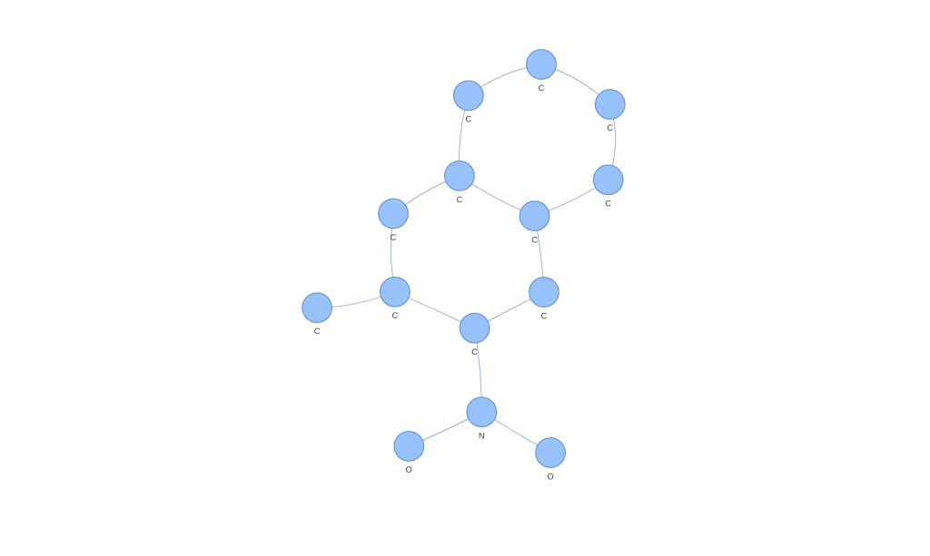
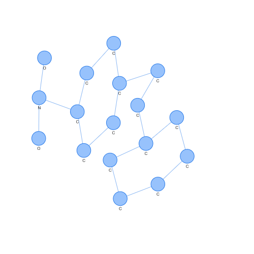
We can even extract those molecular graphs that correspond to support vectors (those points that are used to obtain the hyperplane that the SVM generates) and observe them. For example, the case of a support vector of class 1.
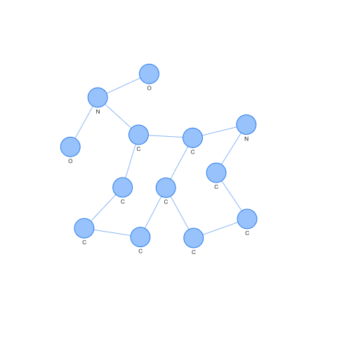
On the contrary, we can see the case of a support vector of class -1. Looking at both, we can easily appreciate differences by eye, but what is interesting is how these differences have been seen in a space where SVM or other popular algorithms can operate.
But we can still experiment more with kernels. For example, there is a very popular kernel which is the RBF (Radial Basis Function) kernel, because it can generate an infinite-dimensional Hilbert space. So, let’s try modifying our Weisfeiler-Lehman kernel to work with the RBF kernel.
In order to do this, it is necessary to move from how the Weisfeiler-Lehman kernel calculates the similarities between two graphs to calculating the dissimilarities. In essence, being the Euclidean distance between the elements belonging to graph A with the elements belonging to graph B, using the name labels of each sub-tree as elements.
The spacing again is different and the visible patterns have changed, although they could well be the same patterns seen previously but expressed differently.
We apply SVM again, with three hyper-parameters to optimize: h, the Weisfeiler-Lehman kernel depth, C the class misclassification penalty and δ, the RBF kernel parameter. Doing a simple search, we obtain the optimal classification with C=100, h=9 and δ=50.
| True 1 | True -1 | |
| Predicted 1 | 8 | 4 |
| Predicted -1 | 1 | 23 |
The result is worse than without applying the Weisfeiler-Lehman kernel with RBF, but, in training, it generally gave better results. This is because there were more dimensions in the space obtained making it more linearly separable, but this has also led to overfitting, which did not occur previously as it was a simpler transformation.
Conclusion
Kernels can transform our data from an arbitrary space to an arbitrary Hilbert space. While, normally, this is usually a transformation from a Euclidean space to a Hilbert space, kernels allow us to work with any space as long as the kernel function satisfies the essential properties of being symmetric and positive semidefinite.
In this post, we have illustrated this using molecular graphs as data operating in a space where one would rarely think that PCA or SVM can be applied, but using the power of kernels, it is possible.
If you found this article interesting, we encourage you to visit the Data Science category to see other posts similar to this one and to share it on social networks. See you soon!
