
Many times the datasets we have available contain a high number of variables and what we are looking for is to be able to explain the relationship between the variables. We can reduce the dimensionality of the dataset by obtaining a smaller number of variables that explain as much information as possible from the original data, and this is where Principal Component Analysis (PCA) comes into play.
PCA is a mathematical method that belongs to the unsupervised learning methods (we do not have a target variable with labels) and one of its functions is to extract useful information from the original variables. This helps us to simplify further analysis such as the representation of the data in two or three dimensions.
The mathematical idea behind it is to get p new orthogonal variables (principal components) and each of them is a linear combination of the m original variables, so that they explain as much of the variability of the original data set as possible.
We will now introduce the definition of eigenvalue and eigenvector for the subsequent explanation of the PCA.
Eigenvalue and eigenvector
We define A as a matrix of dimension mxm and v a vector of dimension 1xm not null, we will say that v is an eigenvector of A if there exists a scalar c such that:
![]()
and c is called the eigenvalue associated with the eigenvector v.
One way to calculate the eigenvalues of the matrix A is by using characteristic polynomials. From the above expression we obtain that v(A-cI) = 0, then it is equivalent to det(A-cI) = 0. The zeros of this polynomial are the eigenvalues of the matrix A.
Subsequently, when we explain the PCA we will see that each principal component is an eigenvector of the covariance matrix and the variance explained of the original data by each principal component is the eigenvalue associated with the eigenvector in question.
PCA procedure
Once we have the intuitive idea of how it works and what the objective of the PCA is, in addition to defining the concepts of eigenvalue and eigenvector, it is time to show the steps for the calculation of the principal components.
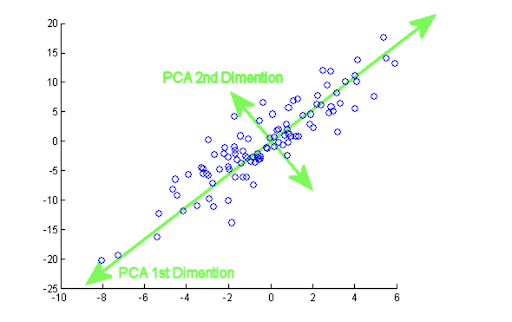
Given a data set X with n observations and p variables, we want there to be an order when obtaining the principal components so that the first component picks up the largest possible variance of the original data, the second component picks up the largest variance not picked up by the first, and so on with the other components.
Since we are trying to pick up as much variance as possible, the variables that have a larger magnitude than others will have a larger scale of variance and, therefore, would dominate over the other variables. To fix this, we will first have to adjust the original variables so that they have a comparable magnitude to each other, thus avoiding the above problem.
Standardization
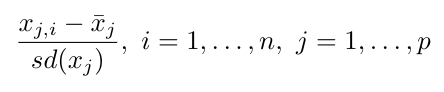
There are different ways of transforming the variables so that they are in the same units, but we are particularly interested in standardizing by subtracting each variable by its mean, and then dividing this difference by its standard deviation:
Calculation of the principal components
Recall that the principal components we are looking for are normalized linear combinations of the original p variables, and at most we can have min{n-1, p} principal components. Suppose we want to construct m principal components, then each of them would look as follows:
![]()
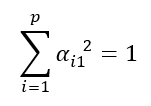
since these are normalized linear combinations, the coefficient vectors of the principal components are unitary or normalized and, therefore, have modulus 1. This condition is reflected in the following constraint:
![]()
The α1j,…,αpj are the loadings of the m-th principal component and each of them marks the weight that each of the p variables has in the component and helps us to collect what type of information each principal component collects.
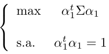
Having all the variables standardized, we can calculate the first component. Theoretically, we try to find the α11,…,αp1 in a way that maximizes the variance of the first principal component:
![]()
The symbol ∑ denotes the covariance matrix of X. This is the function we want to maximize and α11,…,αp1 the variables and the constraint is that:
The formulation of the optimization problem is as follows:
We apply the Lagrange multiplier method and our function to maximize is:
![]()
We derive the function F with respect to the α11,…,αp1 and with a few algebraic manipulations we have the following system of equations in its matrix form:
![]()
To get a non-trivial solution of the problem, α1 non-zero and mandatorily it is the other part that has to be zero. As we explained in the Eigenvalue and Eigenvector section, we realize that λ is an eigenvalue of ∑ with associated eigenvector α1. We calculate the expression of the characteristic polynomial of the covariance matrix and there will be p associated eigenvalues: λ1, λ2,…,λp. The eigenvalue with the largest value will be our solution, since the λ represent the variance of the first principal component. Once the eigenvalue is chosen, we proceed to calculate the associated eigenvector (α1) but we will skip it in order not to extend too much the post.
The calculation of the principal components is performed in a similar way but adding the relevant non-correlation restrictions, since the principal components are orthogonal. An important result is that the sum of the variances of the principal components is equal to the sum of the variances of the original variables, whereby:
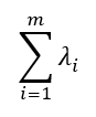
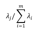
is the total variance of the original data set and the variance explained by the j-th principal component is:
Conclusion
This post is an introduction to Principal Component Analysis and we have given a brief explanation of the mathematical basis behind the method. In the end, to get the principal components we have to solve some optimization problems with the orthogonality and normality constraints of the principal components.
Coming soon
In a future post we will illustrate a small example of using PCA. We will implement in Python a simple example where we will see the code used and some graphics. In particular, we will see how we can interpret the original variables on the axes of the first two principal components.
In the meantime, you can go to the Algorithms category of our blog and see more articles similar to this one.
We encourage you to follow us on Twitter, Linkedin, Facebook e Instagram and share this article with all your contacts. Don’t forget to mention us to let us know what you think, see you soon!
