
The pricing systems currently used in companies have a substantial difference with respect to those of 20 years ago. We have moved from static pricing systems, that is, constant prices at different times of the year, to dynamic systems, where prices can vary according to multiple factors such as demand, competition, available stock and so on.
It is common to deal with this dynamism through complex rule systems that can activate multiple rules for a single day, among which there may be incompatibilities. That is, when control over the rules generated is lost due to their large volume, it is possible that inconsistencies occur, such as certain rules never being able to be executed because they are incompatible with others that have a higher order of importance.
In this article, we will work with a simplified proof of concept to try to identify which rules are feasible and which are not.
Context of the demo
We will work with price rules for two products, A and B, and the dimensions, that is, the fields that determine whether these rules are activated or not, will be the day of the week. However, as we have commented above, the number of dimensions that could cause the rules to be activated can be many and varied.
The days for which we will study which rules should be applied are 2024-06-30, which is a Sunday, and 2024-07-01, which is a Monday.
Types of rules
In this demo we will work with two types of rules: absolute and relative. Absolute rules consist of setting a maximum or minimum price for a certain product. The important nuance is that these rules only contain information of a single product per rule. On the other hand, we will work with relative rules, which, in our demo, refer to two products per rule (two products have been chosen to simplify the demonstration a little, but working with more than two products per rule is not inconvenient).
Each rule has an assigned importance. The interpretation given is that the lower this value, the higher the importance of the rule.
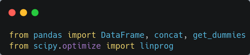
Let’s start by importing the necessary dependencies of the whole demo:
Absolute rules
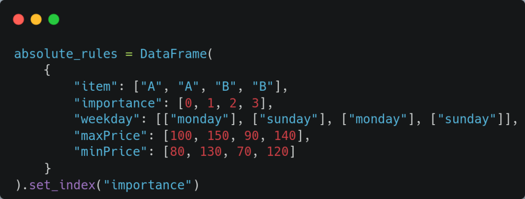
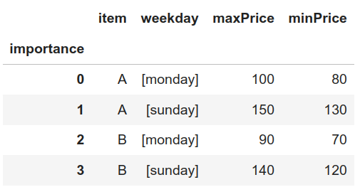
Two absolute rules have been created per product:
- Product A:
- Monday must cost between 80 and 100.
- On Sunday it must cost between 130 and 150.
- Product B:
- Monday must cost between 70 and 90.
- On Sunday it should cost between 120 and 140.
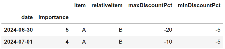
These rules must be processed to identify which ones apply for each day of interest. In our case, the result of this process is as follows:
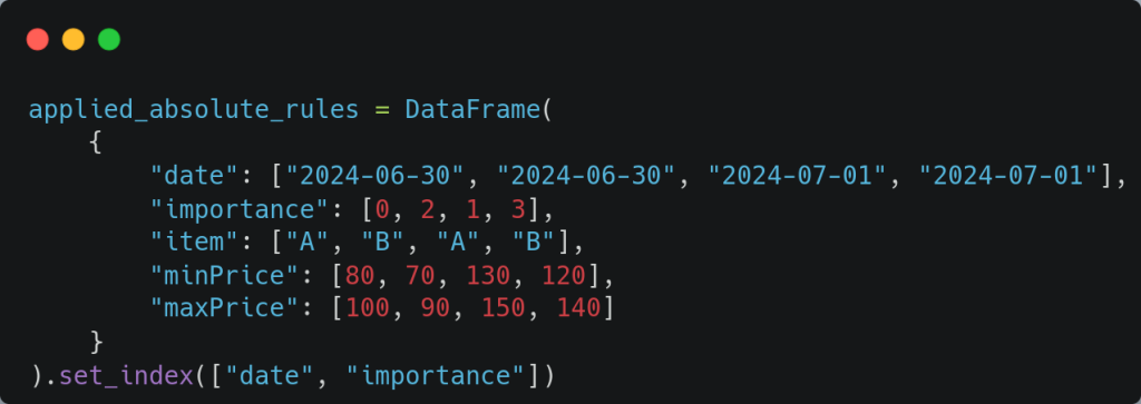
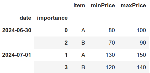
That is, for the interest day 2024-06-30, the absolute rules that apply are those with importance 0 and 2. On the other hand, for the interest day 2024-07-01, the absolute rules that apply are those with importance 1 and 3.
Relative rules
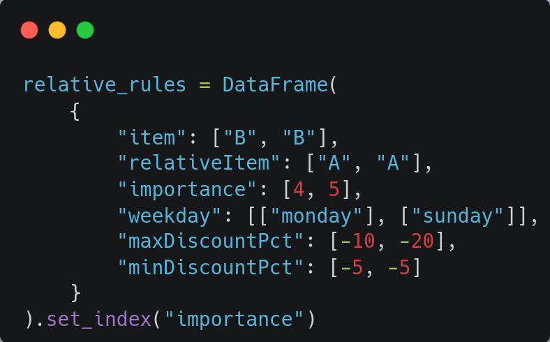
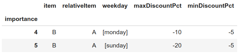
Two relative rules have been created:
- On Mondays, product B must have between 5% and 10% discount with respect to product A. That is, at most product B must cost the price of product A with a 5% discount applied, and at least it must cost the price of product A with a 10% discount applied.
- On Sundays, the above maximum discount percentage increases from 10% to 20%. The minimum discount percentage remains the same as in the previous rule, that is, it is 5%.
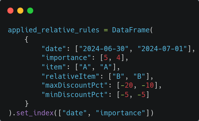
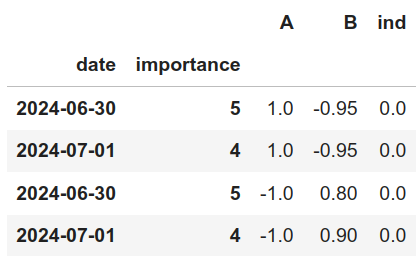
As with the absolute rules, these rules must be processed each day that you want to study which rules apply. In our case, the result of this process is as follows:
Constraint matrix
The constraint matrix is the numerical representation of the rules. It has the following characteristics:
- Each row consists of an inequality rule of type “less than” where on the left of the inequality we have all the terms that depend on the price of a product and on the right of the inequality we have the term that does not depend on the price of any item, also called independent term.
- Each column corresponds to a product whose value is the coefficient that multiplies that product in the inequality.
- There is an additional column corresponding to the independent term of the rule.
In case of having “greater than” type rules, these must be previously rotated to become “less than” type before creating the constraint matrix.
Equality rules must be treated as two inequality rules, one of type “less than” and the other of type “greater than”, where the latter must be transformed to type “less than” before constructing the constraint matrix.
It will be much better understood if we work with examples mentioned above:
- Absolute rule with importance 0 applying day 2024-06-30.
- Mathematically, it can be expressed as 80 <= A <= 100.
- If we separate it into two inequalities we get A > 80 and A <= 100.
- If we express the two inequalities in “less than” format leaving the independent term to the right of the inequality we get -A <= -80 and A <= 100.
- We create the constraint matrix using the coefficients of the two inequalities above, where each row corresponds to an inequality:
| A | B | Independent |
|---|---|---|
| -1 | 0 | -80 |
| 1 | 0 | 100 |
- Relative rule with importance 4 that applies to day 2024-07-01.
- Mathematically, it can be expressed as 0.9 * B <= A <= 0.95 * B.
- If we separate it into two inequalities we get A > 0.9 * B and A <= 0.95 * B.
- If we express the two inequalities in “less than” format leaving the independent term to the right of the inequality we get -A + 0.9 * B <= 0 and A – 0.95 * B <= 0.
- We create the constraint matrix using the coefficients of the two inequalities above, where each row corresponds to an inequality:
| A | B | Independent |
|---|---|---|
| -1 | 0.9 | 0 |
| 1 | 0.95 | 0 |
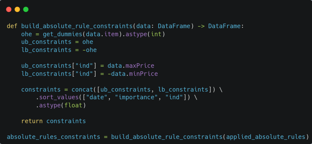
Restriction matrix of absolute rules
The following code converts the object containing the absolute rules that apply per day of interest to a constraint matrix:
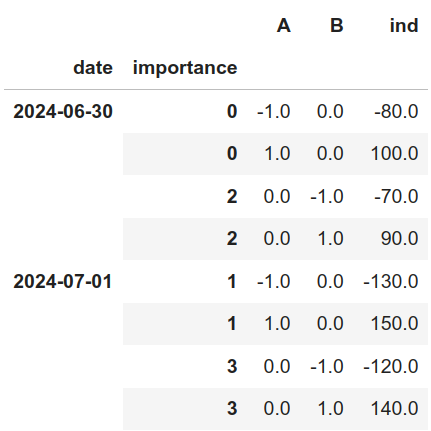
The result is as follows:
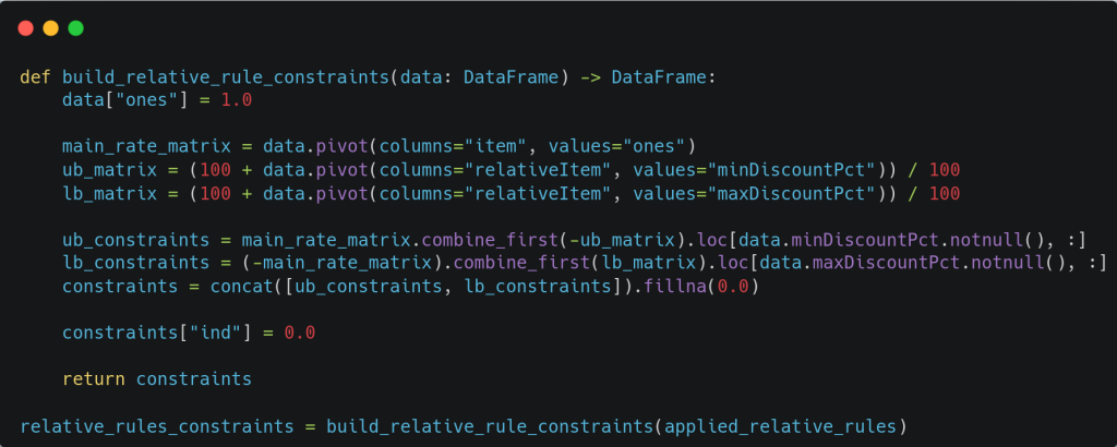
Relative rules constraint matrix
In the same way, the following code converts the object containing the relative rules that apply per day of interest to a constraint matrix:
The result is as follows:
Full constraint matrix
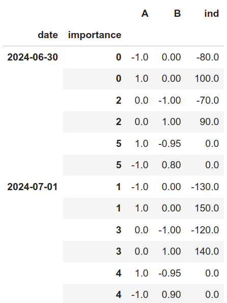
The full constraint matrix is nothing more than the concatenation of the two constraint matrices calculated so far:

Feasible rules
Once we have the constraint matrix calculated, it is time to identify which constraints are infeasible, that is, which cannot be applied if we want to apply the most important ones due to incompatibility.
To solve this problem, we can use linear programming, which is a mathematical procedure for optimizing linear objective functions with linear inequality constraints.
In our context, we do not have an objective function that we want to optimize. We are only interested in whether the constraints allow a solution to exist if an objective function exists.
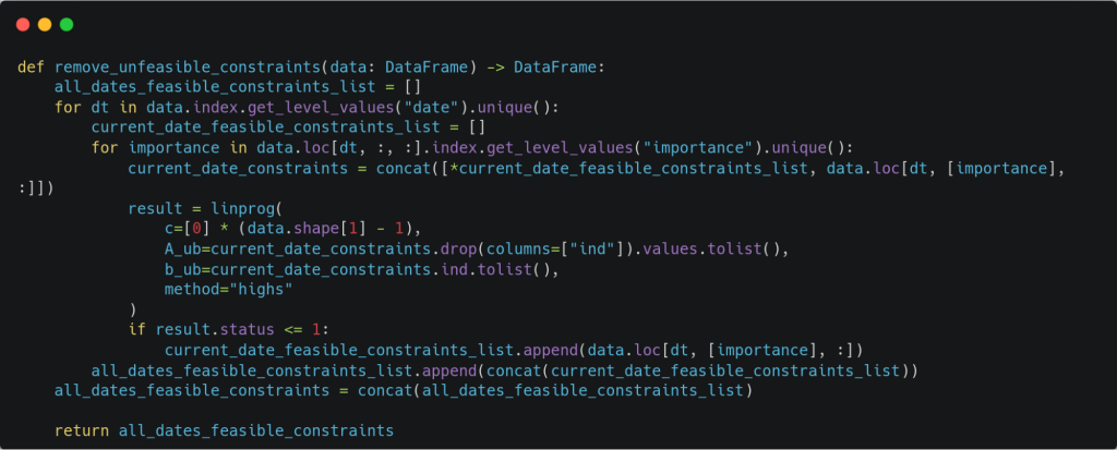
The following code analyzes, by day of interest, each of the calculated constraints and determines whether or not they are feasible. If not, they are discarded. This function returns a constraint matrix that is feasible.
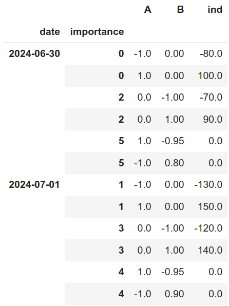
Since the rules we have used so far do not conflict with each other, all the constraints are feasible, so the output of the function is the same as its input in the example we have been working on, which is the following:
Case with infeasible rule
In this example, we add an absolute rule that is inconsistent with the previous ones and with a lower level of importance (it has less priority). This rule specifies that on Mondays product A must cost between 800 and 1000. This rule is inconsistent with the rule that specifies that on Mondays, product A must cost between 130 and 150. For this reason, the new rule added in this example should be discarded by the system.
In this new context, the absolute rules to apply for each day of interest are as follows:
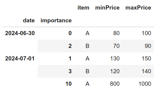
It can be seen that a new row with importance 10 has been added.
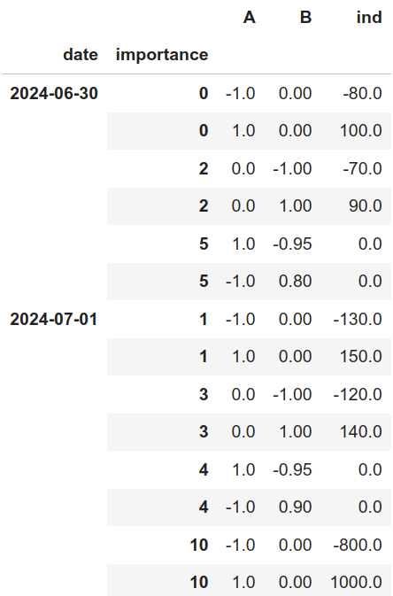
The new constraint matrix is therefore as follows:
If we apply the function again to eliminate infeasible rules:
It will be observed that it returns the same result as when this new rule did not exist, which implies that the system has correctly discarded it.
Conclusion
In this article we have learned how to solve systems of rules that determine which are the feasible price ranges per day and product of interest. By using the mathematical technique Linear Programming we have detected which rules do not allow a solution of the system.
A limitation of this methodology is that it does not apply to contexts in which the rules generate non-linear constraints. In practice this limitation is not frequent, since a common business need is that the pricing rules are easy to interpret, so keeping them linear facilitates their interpretability.
If you found this article interesting, we encourage you to visit the Algorithms category of the blog to see posts similar to this one and to take a look at the Damavis website to learn about real Big Data projects and cases that we have implemented. See you soon!
