
Modeling and explaining the consumer behavior of a product is very important to know what factors affect their behavior, price being one of these important factors.
Let’s take as an example a company X that sells clothing. It is a product that is consumed by many people and there is a large supply in the market and this company adopts the position of raising the prices of its products due to economic problems. For most products this price increase would lead to a decrease in sales as some customers would stop buying, as they could consume other goods or purchase the same item from other cheaper sellers.
The question here is, how much will buyers stop buying? This is where the concept of price elasticity of demand comes in, which quantitatively measures the consumer’s reaction to a change in price.
Price elasticity of demand: Definition
Price elasticity of demand (PE) is a measure that calculates how much of a good is affected by a change in the price of that good. As discussed above, this measure provides quantitative information about consumer behavior when prices change. Generally, the price elasticity of demand is negative following the law of demand (inverse relationship between price and quantity demanded of a good), excluding some luxury or necessity goods that may have a positive elasticity.
The calculation is made as the quotient between the percentage change in quantity demanded and the percentage change in price.
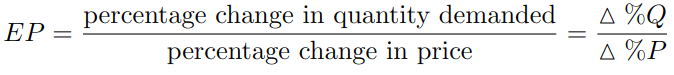
Following the same example of clothing, let’s imagine that increasing the price by 3% decreases the quantity of clothing purchased by 1%, then the elasticity we have in this case would be 3%/-1%=-3. This means that the change in quantity demanded is proportionally 3 times greater than the change in price.
Types of elasticities
According to the value (in absolute value) we can distinguish 3 types of elasticity:
- 0 => EP => -1: Demand is said to be inelastic since the quantity demanded is slightly affected by the change in price.
- EP = -1: Demand is said to be unitary since the quantity demanded is affected proportionally to the change in price.
- EP <= -1: Demand is said to be elastic since the quantity demanded is affected considerably by the change in price.
Factors that can determine elasticity
The price elasticity of demand measures the sensitivity and willingness of the consumer when there is a change in the price of the good, as the demand curve takes into account factors specific to consumer preference beyond price, there are different components that determine the elasticity of the demand curve. Some factors are:
- Availability of alternatives: Goods or products with close substitutes tend to have a more elastic demand, since the good is easily substitutable for another with similar characteristics. An example could be the fruit market, if the price of one fruit goes up, people will tend to buy other fruits.
- Necessity: Necessary goods tend to have inelastic demands, while luxury goods tend to have elastic demands. If the price of electricity is raised, people will continue to need electricity in their homes and may be able to reduce their consumption slightly, but they will not stop using it because it is necessary. On the other hand, if the price of cars is increased, the quantity of cars demanded will fall drastically because it is a less necessary good.
- Market definition: The wider the definition of the good, the lower the elasticity and vice versa. The more defined the market is, the more elastic the demand is due to the presence of substitute goods. Food is a good that defines a broad market and has an inelastic demand, since there are no close substitutes for food. On the other hand, biscuits as a subcategory have an elastic demand, since there are other desserts that could substitute for them.
Constant elasticity approximation
We define a demand with constant elasticity and demand function:
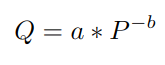
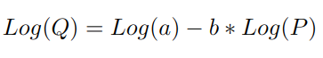
The coefficient that interests us in this case is b, which corresponds to the price elasticity of demand. To do this, we transform the following expression by applying logarithms to both sides of the equality:
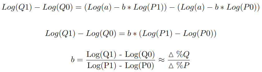
By applying logarithms, the coefficient b is an approximation of the percentage change in Q given a small percentage change in P, which is exactly the definition of the price elasticity of demand given above. Suppose Q0 is the quantity sold at price P0 and Q1 the quantity sold at price P1, to better visualize why b is the price elasticity of demand let’s see what happens when we go from price P0 to P1:
Example with Python
Let’s look at a simple example of how to estimate the elasticity of demand with Python. For this, we will use a dataset on prices and quantities sold of avocados in different US states. The dataset can be downloaded from kaggle.
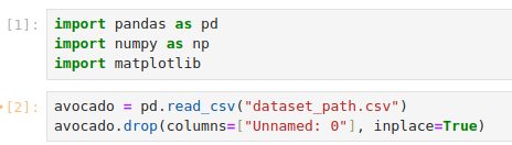
Let’s import the necessary packages and see what the data looks like:
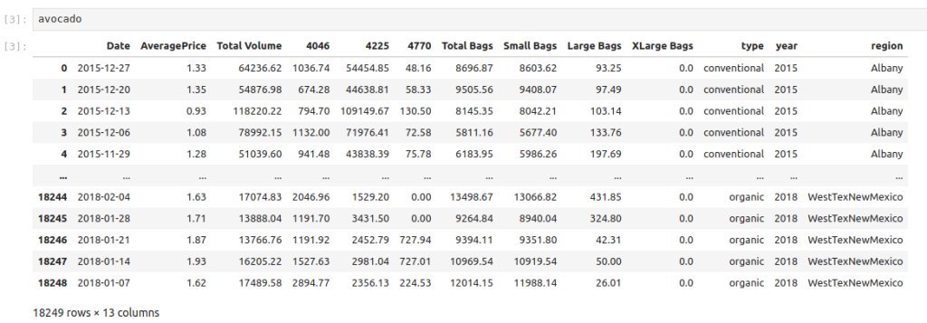
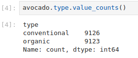
Each row corresponds to a date, the quantities and prices of the avocados that were sold and the US state to which the record corresponds. It can also be seen that the data separates the avocados by type, specifically there are two:
Since the purpose of this section is simply to illustrate a simple and straightforward example of how to estimate the price elasticity of demand with a Python data set, we will select the records corresponding to the state of California and conventional avocados. In addition, let’s see with a scatter plot how is the relationship between quantity demanded and prices.

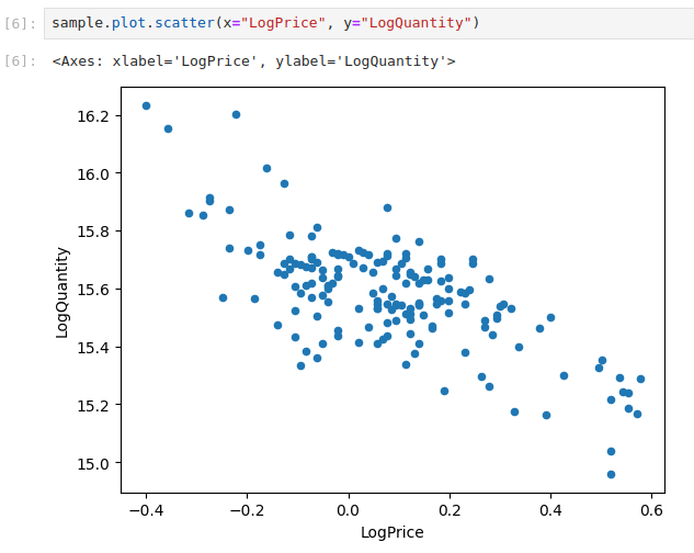
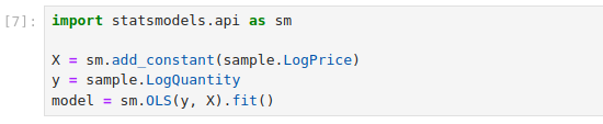
We can see an inverse relationship between the relative change in price and the relative change in quantity demanded, which indicates that the price elasticity of demand has a negative value. To estimate the elasticity we will use the log-log model, as mentioned above, and the estimated coefficient of the explanatory variable LogPrice is the price elasticity of demand.
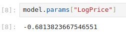
As we suspected, the price elasticity of demand has an approximate value of -0.6814, a 1% increase in price has an impact on demand so that it falls by 0.6814%. It is an inelastic demand and, therefore, a change in price slightly affects the quantity demanded.
Conclusion
In this post we have introduced and defined the concept of price elasticity of demand, an important element of demand to better understand consumer behavior with respect to price changes. We have seen an example of how to estimate the elasticity with a log-log model in Python, the objective has been to illustrate the procedure with a simple example.
That’s it for today’s post. If you found it interesting, we encourage you to visit the Data Science category to see all the related posts and to share it in networks with your contacts. See you soon!
