
When processing data, we often find ourselves in a situation where we want to calculate
variables over certain subset of observations. For example, we might be interested in the
average value per group or the maximum value for each group. Thanks to the use of Window functions, it is possible to perform various calculations on a group of rows related to a specific record.
Throughout this article, we will analyse what Window functions are and how they are used through various practical examples.
How groupBy and Window work
The groupBy function available in many programming or consulting programs allows us to do these calculations easily. To do this, we simply need to specify the variables that define the final group and the functions that we want to apply within each group.
Normally, after applying groupBy, only one observation is obtained for each of the groups are defined. This means that if we want to compare the aggregates obtained with the
observations that generated them, we would have to create a specific function or use a join of the original table with the results of groupBy.
To facilitate tasks like this, many programming languages have the Window function. This function has a similar function to groupBy, with the difference that Window does not modify the number of rows of the DataFrame. In this post we will explain how to use Window in Apache Spark, specifically in its implementation in PySpark.
What is the difference between groupBy and Window in Spark?
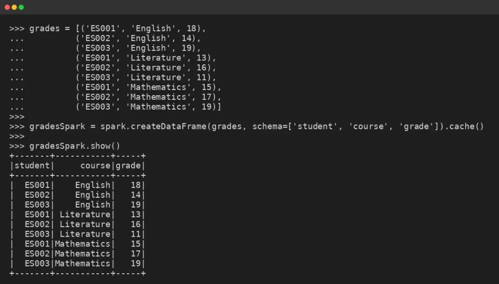
When comparing the behaviour of groupBy with Window, let’s imagine the following problem. We have a set of students and for each one we have the class they were in and the grade obtained. From this data, we want to determine if a student got a grade higher than the average of his class.
First, we will generate some simulated data for testing:
Example of using groupBy
To solve this problem using only groupBy, we first group by class to obtain the average. Then, to match this variable with the original data, we use a join:
~~~~ python
result = gradesSpark.join(gradesSpark.groupBy('course').agg(avg(col('grade')).alias('courseAvg')),
                          on=['course'],
                          how='left')

result = result.withColumn('aboveAvg', when(col('grade')>col('courseAvg'), lit(1)).otherwise(lit(0)))

result.show()
~~~~

~~~~ console
+-------+-------+-----+------------------+--------+
| course|student|grade|         courseAvg|aboveAvg|
+-------+-------+-----+------------------+--------+
|English|  ES001|   18|              17.0|       1|
|English|  ES002|   14|              17.0|       0|
|English|  ES003|   19|              17.0|       1|
| French|  ES001|   13|13.333333333333334|       0|
| French|  ES002|   16|13.333333333333334|       1|
| French|  ES003|   11|13.333333333333334|       0|
|  Maths|  ES001|   15|              17.0|       0|
|  Maths|  ES002|   17|              17.0|       0|
|  Maths|  ES003|   19|              17.0|       1|
+-------+-------+-----+------------------+--------+
~~~~
How to use Window function
When using Window with this same example, the process is much simpler. We only need to define the window in which we want to apply the function and then create the variable using the over(), indicating the window we want to use for the calculation:
~~~~ python
win = Window.partitionBy('course')

result = gradesSpark.withColumn('courseAvg', avg(col('grade')).over(win))

result = result.withColumn('aboveAvg', when(col('grade')>col('courseAvg'), lit(1)).otherwise(lit(0)))

result.show()
~~~~

~~~~ console
+-------+-------+-----+------------------+--------+
|student| course|grade|         courseAvg|aboveAvg|
+-------+-------+-----+------------------+--------+
|  ES003|English|   19|              17.0|       1|
|  ES001|English|   18|              17.0|       1|
|  ES002|English|   14|              17.0|       0|
|  ES001| French|   13|13.333333333333334|       0|
|  ES002| French|   16|13.333333333333334|       1|
|  ES003| French|   11|13.333333333333334|       0|
|  ES001|  Maths|   15|              17.0|       0|
|  ES002|  Maths|   17|              17.0|       0|
|  ES003|  Maths|   19|              17.0|       1|
+-------+-------+-----+------------------+--------+
~~~~
As you can see, the code with Window is much less complicated and more efficient. This is because there is no need to do a join, which can often be very computationally expensive.
Type of Windows in Apache Spark
Apache Spark offers different functions that we can combine to sit many window types easily. Below, we will analyse some of them.
Using partitionBy
In this case, partitionBy is what we used in the previous example and serves to define the groups that we have inside the data. This function requires a list with the variables that delimit such groups as when we use a groupBy.
How to use orderBy
As is name suggest, orderBy allow us to organise the data within a group. In addition, when using orderBy alone or with partitionBy when defining the window, the calculations are performed for all rows whose value precedes or is equal to that of the current row. This way, if two rows have the same value for the variable being ordered, both will enter the calculation.
Example of using orderBy
To exemplify the use of orderBy, we will use data on the contribution of different sectors to GDP. In this example, we will imagine that we want to keep the largest sectors whose combined contribution is at least 80%. To do this, we can use a window with orderBy, define a descending order according to the percentage of GDP, and sum up:
~~~~ python
gdp = [('Agriculture', 5),
       ('Telecom', 25),
       ('Tourism', 40),
       ('Petrochemical', 25),
       ('Construction', 5)]

gdpSpark = spark.createDataFrame(gdp, schema=['sector', 'percGdp'])

win = Window().orderBy(col('percGdp').desc())
win2 = Window().orderBy(col('percGdp').desc()).rowsBetween(Window.unboundedPreceding, Window.currentRow)


gdpSpark.withColumn('percBiggerSectors', sum(col('percGdp')).over(win)).show()
~~~~

~~~~ console
+-------------+-------+-----------------+
|       sector|percGdp|percBiggerSectors|
+-------------+-------+-----------------+
|      Tourism|     40|               40|
|      Telecom|     25|               90|
|Petrochemical|     25|               90|
| Construction|      5|              100|
|  Agriculture|      5|              100|
+-------------+-------+-----------------+
~~~~
As can be seen, Telecommunications the value of percBiggerSectors is 90=40+25+25. In this sense, orderBy does not take into account that Petrochemical is in the next row, but that the value 25 is the same in both rows. Another important feature that emerges from this example is that it is not necessary to use partitionBy together with orderBy. If partionBy is not included, in the group is simply all data.
On the other hand, orderBy is also useful when we want to use order to create variables. For example, with the grade data we used in the previous section, we could create a ranking of students according to their grade within each class:
~~~~ python
win = Window.partitionBy('course').orderBy(col('grade').desc())

result = gradesSpark.withColumn('ranking', rank().over(win))

result.show()
~~~~

~~~~ console
+-------+-------+-----+-------+
|student| course|grade|ranking|
+-------+-------+-----+-------+
|  ES003|English|   19|      1|
|  ES001|English|   18|      2|
|  ES002|English|   14|      3|
|  ES002| French|   16|      1|
|  ES001| French|   13|      2|
|  ES003| French|   11|      3|
|  ES003|  Maths|   19|      1|
|  ES002|  Maths|   17|      2|
|  ES001|  Maths|   15|      3|
+-------+-------+-----+-------+
~~~~
Using the rowsBetween function
This function helps us define dynamic windows that depend on the row in which a calculation is being made. It requires two elements that indicate the beginning and the end of the dynamic window. These two values are integers relative to the current row, for example rowsBetween(-1, 1) would indicate that the window goes from the row before the current row to the row after the current row.
However, Apache Spark provides and recommends using, where possible, several functions to define these intervals, in order to minimise human error and increase the readability of the code:
- currentRow indicates the current row where the calculation is being performed.
- unboundedPreceding refers the first row of the group.
- unboundedFollowing indicates the last row of the group.
How rowsBetween works
To observe how rowsBetween works, let’s assume we have the following data about the
price of a stock:
~~~~ python
prices = [('AAPL', '2021-01-01', 110),
          ('AAPL', '2021-01-02', 120),
          ('AAPL', '2021-01-03', 110),
          ('AAPL', '2021-01-04', 115),
          ('AAPL', '2021-01-05', 150),
          ('MSFT', '2021-01-01', 150),
          ('MSFT', '2021-01-02', 130),
          ('MSFT', '2021-01-03', 140),
          ('MSFT', '2021-01-04', 120),
          ('MSFT', '2021-01-05', 140)]

pricesSpark = spark.createDataFrame(prices, schema=['company', 'date', 'price'])\
                    .withColumn('date', to_date(col('date'))).cache()


pricesSpark.show()
~~~~

~~~~ console
+-------+----------+-----+
|company|      date|price|
+-------+----------+-----+
|   AAPL|2021-01-01|  110|
|   AAPL|2021-01-02|  120|
|   AAPL|2021-01-03|  110|
|   AAPL|2021-01-04|  115|
|   AAPL|2021-01-05|  150|
|   MSFT|2021-01-01|  150|
|   MSFT|2021-01-02|  130|
|   MSFT|2021-01-03|  140|
|   MSFT|2021-01-04|  120|
|   MSFT|2021-01-05|  140|
+-------+----------+-----+
~~~~
Example of rowsBetween
If we want to calculate a moving average from the first date to the date in the current row, we could do the following in the current row:
~~~~ python
win = Window.partitionBy('company').orderBy('date').rowsBetween(Window.unboundedPreceding, Window.currentRow)
win2 = Window.partitionBy('company').orderBy('date')

pricesSpark.withColumn('histAvg', avg(col('price')).over(win))\
            .withColumn('histAvg2', avg(col('price')).over(win2)).show()
~~~~

~~~~ console
+-------+----------+-----+------------------+------------------+
|company|      date|price|           histAvg|          histAvg2|
+-------+----------+-----+------------------+------------------+
|   AAPL|2021-01-01|  110|             110.0|             110.0|
|   AAPL|2021-01-02|  120|             115.0|             115.0|
|   AAPL|2021-01-03|  110|113.33333333333333|113.33333333333333|
|   AAPL|2021-01-04|  115|            113.75|            113.75|
|   AAPL|2021-01-05|  150|             121.0|             121.0|
|   MSFT|2021-01-01|  150|             150.0|             150.0|
|   MSFT|2021-01-02|  130|             140.0|             140.0|
|   MSFT|2021-01-03|  140|             140.0|             140.0|
|   MSFT|2021-01-04|  120|             135.0|             135.0|
|   MSFT|2021-01-05|  140|             136.0|             136.0|
+-------+----------+-----+------------------+------------------+
~~~~
Note that using the win window or the win 2 window it gives the same result. In this case, there are no repeated dates within each group, so the behaviour of orderBy does not manifest itself. However, if we use the example with data from the GDP we notice that when using rowsBetween, the data used to calculate the sum is only up to the current row. Therefore, in histAvg2 the Telecommunication value is only 65 = 40 + 25:
~~~~ python
win = Window().orderBy(col('percGdp').desc())
win2 = Window().orderBy(col('percGdp').desc()).rowsBetween(Window.unboundedPreceding, Window.currentRow)

gdpSpark.withColumn('percBiggerSectors', sum(col('percGdp')).over(win))\
        .withColumn('percBiggerSectors2', sum(col('percGdp')).over(win2)).show()
~~~~

~~~~ console
+-------------+-------+-----------------+------------------+
|       sector|percGdp|percBiggerSectors|percBiggerSectors2|
+-------------+-------+-----------------+------------------+
|      Tourism|     40|               40|                40|
|      Telecom|     25|               90|                65|
|Petrochemical|     25|               90|                90|
|  Agriculture|      5|              100|                95|
| Construction|      5|              100|               100|
+-------------+-------+-----------------+------------------+
~~~~
How rangeBetween works
This function is similar to rowsBetween but works with the values of the variable used inside orderBy instead of the rows. A window created with rangeBetween has the same behaviour as when using orderBy alone, but it allows us to define a different range and not only from the first value to the current one. It receives two arguments that indicate how many values below and above the current value you want within the window.
For example, let’s day that for one row, the salary is 10 euros and there is a window defined by window.orderBy(‘salary’).rangeBetween(-5, 5). If we carry out a calculation on this window, the set that will be taken into account for this row will be all the rows whose wages are between 5 and 15 euros.
Let’s go back to the example of the students. When working with this data, we might want to compare them with those students who get similar grades. For example, we could compare them with the average of their class, but only those students who get +-2 points more than them. Using rangeBetween, the code would be:
~~~~ python
win = Window.partitionBy('course').orderBy('grade').rangeBetween(-2, 2)

result = gradesSpark.withColumn('similarStudentsAvg', mean(col('grade')).over(win))

result = result.withColumn('aboveAvg', when(col('grade')>=col('similarStudentsAvg'), lit(1)).otherwise(lit(0)))

result.show()
~~~~

~~~~ console
+-------+-------+-----+------------------+--------+
|student| course|grade|similarStudentsAvg|aboveAvg|
+-------+-------+-----+------------------+--------+
|  ES002|English|   14|              14.0|       1|
|  ES001|English|   18|              18.5|       0|
|  ES003|English|   19|              18.5|       1|
|  ES003| French|   11|              12.0|       0|
|  ES001| French|   13|              12.0|       1|
|  ES002| French|   16|              16.0|       1|
|  ES001|  Maths|   15|              16.0|       0|
|  ES002|  Maths|   17|              17.0|       1|
|  ES003|  Maths|   19|              18.0|       1|
+-------+-------+-----+------------------+--------+
~~~~
Functions to create variables with windows
In Apache Spark, we can divide the functions that can be used on a window into two main groups. In addition, users can define their own functions, just like when using groupBy (the use of udfs should be avoided as they tend to perform very poorly).
What are analytical functions?
Analytical functions return a value for each row in a set that may be different for each row. Below, we analyse the different types that exist.
Types of analytical functions
- rank. Allows us to assign to each row within a group a natural number that indicates the place the row has according to the value of the variable used in the orderBy. If two rows are tied, they are assigned the same number in the rank and a number is skipped for the next row.
- denseRank. It has the same purpose as rank only that when there are ties a number is not skipped for the row after the tied rows.
- percentRank. Gives us the percentile that corresponds to the row when the data is sorted according to the variable used in orderBy.
- rowNumber. Allows us to assign to each row within a group a different natural number that indicates the place that the row has according to the value of the variable used in the orderBy. If two rows are tied the ranking is assigned randomly so the results are not always equal.
- nTile(n). Used to distribute the rows of a group among n groups. It is very useful when you want to make an ordinal variable from a numeric variable; for example 4 income levels with the same number of observations each.
- lag(col, n, default). Gives us the value of the column
col, n rows before the current row. If n is a negative number it implies that we get the value that the columncol, n rows after the current row has. If the group does not have enough rows before or after the current row lag returns nan unless the function is called with the optional parameter default in which case it will return said value. The order of the rows is given by the column used in the window’s orderBy so when using lag it is necessary that the window contains this clause. - lead(col, n, default). Same as lag only that positive numbers imply later rows and
negative numbers earlier rows. - cumeDist. Gives the cumulative probability of each row according to the variable used in orderBy. In other words, it tells us the proportion of rows whose value in the variable used in orderBy is less than or equal to the value of that variable for the current row.
- last(col, ignorenulls). Returns the last value observed in the col column before the current row within the specified window. Requires the window to have an orderBy. The argument ignorenulls=True allows ignoring all missing values which causes the first non-null value before the current row to be returned.
Aggregation functions
All the functions that compact a set of data into a single value that represents the set, such as sum, min, max, avg and count functions.
Additional usage examples
Using rangeBetween and window dates
If you want to apply rangeBetween to create window dates, simply transform the dates to timestamp and divide by the number of seconds in the period we want to calculate the window. For example, dividing by 86400 for days or 3600 for hours. In the following example, if we wanted to find the three day moving average we couldn’t use rowsBetween as before. This is because we have missing dates but we can use rangeBetween:
~~~~ python
prices2 = [('AAPL', '2021-01-05', 110),
           ('AAPL', '2021-01-07', 120),
           ('AAPL', '2021-01-13', 110),
           ('AAPL', '2021-01-14', 115),
           ('AAPL', '2021-01-15', 150),
           ('MSFT', '2021-01-01', 150),
           ('MSFT', '2021-01-05', 130),
           ('MSFT', '2021-01-06', 140),
           ('MSFT', '2021-01-09', 120),
           ('MSFT', '2021-01-12', 140)]

pricesSpark2 = spark.createDataFrame(prices2, schema=['company', 'date', 'price'])\
                     .withColumn('date', to_date(col('date'))).cache()

pricesSpark2.show()
~~~~

~~~~ console
+-------+----------+-----+
|company|      date|price|
+-------+----------+-----+
|   AAPL|2021-01-05|  110|
|   AAPL|2021-01-07|  120|
|   AAPL|2021-01-13|  110|
|   AAPL|2021-01-14|  115|
|   AAPL|2021-01-15|  150|
|   MSFT|2021-01-01|  150|
|   MSFT|2021-01-05|  130|
|   MSFT|2021-01-06|  140|
|   MSFT|2021-01-09|  120|
|   MSFT|2021-01-12|  140|
+-------+----------+-----+
~~~~

~~~~ python
days = lambda i: i * 86400
win = Window.partitionBy('company')\
            .orderBy(col('date').cast("timestamp").cast("long"))\
            .rangeBetween(-days(3), 0)

pricesSpark2.withColumn('movingAvg3d', avg(col('price')).over(win)).show()
~~~~

~~~~ console
+-------+----------+-----+-----------+
|company|      date|price|movingAvg3d|
+-------+----------+-----+-----------+
|   AAPL|2021-01-05|  110|      110.0|
|   AAPL|2021-01-07|  120|      115.0|
|   AAPL|2021-01-13|  110|      110.0|
|   AAPL|2021-01-14|  115|      112.5|
|   AAPL|2021-01-15|  150|      125.0|
|   MSFT|2021-01-01|  150|      150.0|
|   MSFT|2021-01-05|  130|      130.0|
|   MSFT|2021-01-06|  140|      135.0|
|   MSFT|2021-01-09|  120|      130.0|
|   MSFT|2021-01-12|  140|      130.0|
+-------+----------+-----+-----------+
~~~~
Example with time series models
On the other hand, if we have a dataset that has no missing dates then obtaining a lagged variable is as simple as using lag with the desired window. Let’s exemplify by applying this procedure to the set of pricesSpark:
~~~~ python
days = lambda i: i * 86400
win = Window.partitionBy('company')\
            .orderBy(col('date').cast("timestamp").cast("long"))
pricesSpark2.withColumn('price_1', lag(col('price')).over(win)).show()
~~~~

~~~~ console
+-------+----------+-----+-------+
|company|      date|price|price_1|
+-------+----------+-----+-------+
|   AAPL|2021-01-05|  110|   null|
|   AAPL|2021-01-07|  120|    110|
|   AAPL|2021-01-13|  110|    120|
|   AAPL|2021-01-14|  115|    110|
|   AAPL|2021-01-15|  150|    115|
|   MSFT|2021-01-01|  150|   null|
|   MSFT|2021-01-05|  130|    150|
|   MSFT|2021-01-06|  140|    130|
|   MSFT|2021-01-09|  120|    140|
|   MSFT|2021-01-12|  140|    120|
+-------+----------+-----+-------+
~~~~
However, in the case of the dataset pricesSpark2 it’s not possible to implement this
methodology since the value of the previous row can correspond to either 1 day before or several days before. In this case, we could use any aggregation function (e.g. sum) together with a window containing rangeBetween to limit the dates on which the function is calculated to exactly the number of previous days we want:
~~~~ python
days = lambda i: i * 86400
win = Window.partitionBy('company')\
            .orderBy(col('date').cast("timestamp").cast("long"))\
            .rangeBetween(-days(1),-days(1))
pricesSpark2.withColumn('price_1', sum(col('price')).over(win)).show()
~~~~

~~~~ console
+-------+----------+-----+-------+
|company|      date|price|price_1|
+-------+----------+-----+-------+
|   AAPL|2021-01-05|  110|   null|
|   AAPL|2021-01-07|  120|   null|
|   AAPL|2021-01-13|  110|   null|
|   AAPL|2021-01-14|  115|    110|
|   AAPL|2021-01-15|  150|    115|
|   MSFT|2021-01-01|  150|   null|
|   MSFT|2021-01-05|  130|   null|
|   MSFT|2021-01-06|  140|    130|
|   MSFT|2021-01-09|  120|   null|
|   MSFT|2021-01-12|  140|   null|
+-------+----------+-----+-------+
~~~~
Calculate the time elapsed since an event
In many situations, we find ourselves with datasets where in each row we have an event and we want to know the date between some of them. For example, we could have a dataset with the logs of certain machines along with the failures they have had:
~~~~ python
events = [('m1', '2021-01-01', 'e1'),
          ('m1', '2021-02-02', 'e1'),
          ('m1', '2021-03-03', 'e2'),
          ('m1', '2021-03-04', 'critical'),
          ('m1', '2021-07-05', 'e1'),
          ('m2', '2021-01-01', 'e1'),
          ('m2', '2021-06-02', 'critical'),
          ('m2', '2021-08-03', 'e2'),
          ('m2', '2021-09-04', 'e1'),
          ('m2', '2021-10-17', 'critical'),
          ('m2', '2021-10-25', 'e1')]

eventsSpark = spark.createDataFrame(events, schema=['machine', 'date', 'error'])\
                   .withColumn('date', to_date(col('date'))).cache()

eventsSpark.show()
~~~~

~~~~ console
+-------+----------+--------+
|machine|      date|   error|
+-------+----------+--------+
|     m1|2021-01-01|      e1|
|     m1|2021-02-02|      e1|
|     m1|2021-03-03|      e2|
|     m1|2021-03-04|critical|
|     m1|2021-07-05|      e1|
|     m2|2021-01-01|      e1|
|     m2|2021-06-02|critical|
|     m2|2021-08-03|      e2|
|     m2|2021-09-04|      e1|
|     m2|2021-10-17|critical|
|     m2|2021-10-25|      e1|
+-------+----------+--------+
~~~~
If we are interested in the time that has elapsed from each of the error types to a critical error we could use the last function along with some auxiliary variables that have missing values unless the error is of a certain type:
~~~~ python
errors = ['e1', 'e2']

# We create variables that have a value if the error is of a certain type
for i in errors:
    eventsSpark = eventsSpark.withColumn('date_'+i, when(col('error')==i, col('date')).otherwise(None))


# We calculate the time from each type of error until a critical error
win = Window.partitionBy('machine').orderBy('date')
for i in errors:
    eventsSpark = eventsSpark.withColumn('daysFromLast_'+i, last(col('date_'+i), True).over(win))\
                             .withColumn('daysFromLast_'+i,
                                         (unix_timestamp(col('date'))-unix_timestamp(col('daysFromLast_'+i)))/86400)

eventsSpark.filter(col('error')=='critical').show()
~~~~

~~~~ console
+-------+----------+--------+-------+-------+-----------+-----------+-----------+-----------+---------------+---------------+
|machine|      date|   error|date_e1|date_e2|dateLast_e1|timeLast_e1|dateLast_e2|timeLast_e2|daysFromLast_e1|daysFromLast_e2|
+-------+----------+--------+-------+-------+-----------+-----------+-----------+-----------+---------------+---------------+
|     m1|2021-03-04|critical|   null|   null| 2021-02-02|       30.0| 2021-03-03|        1.0|           30.0|            1.0|
|     m2|2021-06-02|critical|   null|   null| 2021-01-01|      152.0|       null|       null|          152.0|           null|
|     m2|2021-10-17|critical|   null|   null| 2021-09-04|       43.0| 2021-08-03|       75.0|           43.0|           75.0|
+-------+----------+--------+-------+-------+-----------+-----------+-----------+-----------+---------------+---------------+
~~~~
Conclusion
In this post we have learned what are windows in Spark, the syntax for their definition and the most common functions used with them. In addition, we have seen examples of tasks that can be solved with windows as well as the advantages of its use.
In future posts we will talk about how to define a simple demand model and a recursive strategy to find the optimal selling price. In the meantime, we encourage you to visit the Data Science category of the Damavis blog and see other articles similar to this one.
We invite you to share this article with your friends. Remember to tag us to let us know what you think about it (@DamavisStudio). See you on Networks!
