
In the world of data science and analysis, time series are a key element, as they represent a very natural source of information: values of a magnitude at different points in time. This is why understanding their properties and knowing how to work with them is necessary to successfully develop projects in these fields.
In this post, we are going to focus on the properties of time series that result from comparing and relating them to other time series.
Key concepts
With very high probability, the first thing that comes to mind when talking about relating different time series is to evaluate to what extent “they are the same” or at least “they have the same trend”. Of course, this measure is very relevant and there are a large number of metrics to measure this, some as fundamental and recognized as correlation in its most basic definition.
But suppose for a moment that two time series are exactly the same, but one is lagged by any number of time units. If we were to visually assess the situation, we would say that they are the same time series “just shifted”, but the algorithms mentioned above will not return a value that indicates this so clearly.
Understanding when this happens is very important, as it can also answer questions about the relationship between time series that are extremely relevant: Does a certain variable have predictive power over another? Or even, does a certain variable affect the behavior of another? To find this out at a mathematical level, of course, an algorithm must be introduced that is capable of doing so. One of the best known is “Granger causality“, and in this post we are going to introduce and explain this method.
A brief history
The Granger causality method was introduced in 1969 by the economist and winner of the Nobel Prize for literature in 2003, Sir Clive William John Granger, in his famous article entitled: Investigating causal relations by econometric models and cross-spectral methods.
The initial area of application of this methodology was economics. However, more than 50 years after its introduction, the fields of knowledge in which it has been used have only increased. So much so that today applications of this algorithm can be found in a wide range of fields, from neuroscience to air transport, climatology and meteorology.
The fact that, after so long, this methodology is still being used and that it is becoming increasingly interdisciplinary is further proof of its correct functioning and applicability.
Qualitative idea
The qualitative idea behind this algorithm is that a time series Y “causes” another time series X, if additionally knowing past values of Y (with respect to values of X that we are going to try to predict) improves the prediction of values of X, with respect to only using past values of X.
It is very important to understand why we have used inverted commas when we have written the word cause: the term cause, if we were to use it in a literal sense, in this context would imply that if the aforementioned causality exists, there is something in the magnitude that Y represents that is directly affecting the magnitude that X represents, which means that knowing past values of Y makes it possible to better understand how X evolves.
As it is a mathematical algorithm, this cause-effect relationship is not assured under any circumstances, even if it concludes the existence of causality. To take a very trivial example, two speakers can be independently configured to emit the same signal, one of them with a one-second delay; and while there is no cause-effect relationship between the two, this algorithm will detect causality.
The reason the term causality is used is because it is consistent with the nomenclature proposed by its author, and for compactness in notation; but the term “predictive ability” in this context is probably much more appropriate. In this way, when we say Y causes X, we are in fact saying that Y has predictive capacity over X.
Mathematical implementation
Having understood the qualitative idea behind the algorithm, it is time to introduce the mathematical framework of this methodology that will allow us to implement it with real time series.
Before starting, it is necessary to mention that the methodology to be presented in this post is the one originally introduced by C. W. J. Granger in his original article; but it is not the only existing development.
Analyzing the qualitative idea presented in the previous paragraph, in order to be able to apply it, we have to be able to mathematically evaluate how well the values of X are predicted using both past values of X and Y; and only past values of X. To do this, we will generate two regression models.
First, when we use the two time series:
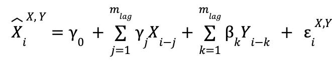
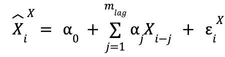
and when we only use past data from X:
![]()
![]() is the value we predict for the i-th element of the time series X, and the superindex indicates which time series the past values we are using (in the variable used for the explanation) are from,
is the value we predict for the i-th element of the time series X, and the superindex indicates which time series the past values we are using (in the variable used for the explanation) are from, ![]() would be X and Y).
would be X and Y).
![]()
![]() is the value at the time step
is the value at the time step ![]() of time series X.
of time series X. ![]() is the error made in the prediction of, for this case, the value
is the error made in the prediction of, for this case, the value ![]() , where the meaning of the superscript and subscript are the same in these two variables. The summations go up to
, where the meaning of the superscript and subscript are the same in these two variables. The summations go up to ![]() , which is the number of past values to be taken to make the predictions (in other words, the number of time units that the most past value used in the predictions will have with respect to the value to be predicted). The value of this parameter is not fixed in advance and is modifiable.
, which is the number of past values to be taken to make the predictions (in other words, the number of time units that the most past value used in the predictions will have with respect to the value to be predicted). The value of this parameter is not fixed in advance and is modifiable.
Finally, the α, β and γ are the parameters to be adjusted, so they do not have a pre-set value either. In order to distinguish between the two models, and bearing in mind that the one that only uses data from the time series X is a specific case of the one that uses both (taking in the former all β as 0 we return to the former), we are going to call the former “restricted model” and the latter “unrestricted model”.
We have commented that there are certain parameters whose value has to be found. According to the original theory presented by Granger, the most optimal predictions of each of the models are those that minimize the variance of the errors made in the predictions, respectively. Mathematically, this variance takes the expression:
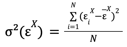
where the summation runs through the errors of all the predictions that have been made with the model for which the variance of the error of values of the time series X is to be calculated (restricted model in the case of the example given), and which in the formula have been assumed to be N. ![]()
![]() is the mean of the errors.
is the mean of the errors.
In general, this last mean will always be able to take the value of 0 (and, although it is not necessary at this point, we will see that for a necessary evaluation of this model, it is), because if it does not take this value, what it is indicating is that there is a constant bias in the model (on average, all the predictions are wrong by a certain value), something that is solved by adding this same value to the independent term of the model.
Under this casuistry, minimizing the variance is equivalent to minimizing the sum of the squares of the errors and, therefore, the error made in the predictions. The parameter sets α, β and γ are those that are adjusted, respectively for each model, to achieve the aforementioned minimization. There is still one last parameter to be set, which would be ![]()
![]() , but for the moment we will not mention how its value is determined, and we will simply assume that it takes any value, that is, greater than or equal to 1.
, but for the moment we will not mention how its value is determined, and we will simply assume that it takes any value, that is, greater than or equal to 1.
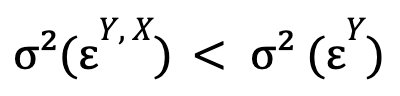
Following C. W. J. Granger’s explanation, we will say that time series Y causes time series X if:
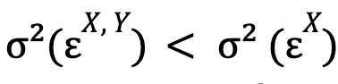
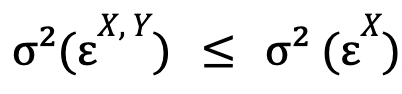
that is, if the optimized error variance for the unconstrained model is smaller than this same magnitude for the constrained model. If additionally also it is verified:
(that is, time series X causes time series Y), we will say that there is feedback between these two time series.
Before concluding this section, it is very important to mention a series of restrictions that this algorithm has. The first one is that, in order to be able to work with this methodology, it is necessary that both time series we are working with are stationary.
Since it is not the aim of this post, the formal explanation of when a time series is stationary and how to check it will not be explained, but a qualitative idea of it and the reason why it is necessary in this methodology will be mentioned. A time series is stationary if its properties (such as its variance) are not a function of time; that is, when calculations are made for different intervals of the time series, the values obtained for the representative magnitudes are the same.
The reason why we need them to be the same in order to apply Granger causality is that, if they were not, properties such as, for example, the variance of the error that we use to draw a conclusion, we cannot be sure that they will not vary over time and, therefore, we would not be able to conclude anything.
The second constraint is that to maximize the reliability of the algorithm, the time series cannot have missing data, that is, they have to have a value assigned to each time step.
Statistical interpretation
If one starts to put into practice what is explained in the previous paragraph, by testing different pairs of stationary time series, one would quickly realize that, very suspiciously, in practically all cases, the mentioned causality (and more specifically feedback) between the pairs of time series occurs.
Of course, it is not that all these causalities are actually happening. What actually happens is that, as we will now see, in the assessment outlined in the previous paragraph, the proposed models themselves, by construction, are practically ensuring that the causality condition is always satisfied.
As we mentioned in the last section, the regression model when using only one time series is a specific case of the unrestricted regression model. So, the unrestricted model will always have a lower error variance or, in the worst case, the same if the minimization of this magnitude in the former is achieved when ![]()
![]() (in which case both optimised models would be the same, i.e.
(in which case both optimised models would be the same, i.e. ![]() ), so that by construction we will always have (for the case where we study whether Y causes X):
), so that by construction we will always have (for the case where we study whether Y causes X):
where, moreover, equality is a highly improbable extreme case.
To solve this problem, the qualitative change we have to make when evaluating the results is to move from answering the question: Can I predict better values of X by also using past values of Y? Which we already know that the answer will always be yes (or at least as good), to answering the question: Does my prediction using also Y values improve enough compared to the one using only X values, considering that in the latter we double both the parameters to be adjusted and the values used?
In order to answer this last question we have to move to a more statistical context. The intuitive idea is that if the predictive power of the second time series over the first is low, all coefficients will be very close to zero, where this closeness will be assessed in terms of how easy it is for the unconstrained model to achieve better predictions than the constrained one.
This is why the statistical test we are going to propose takes as the null hypothesis: All the coefficients β of the unrestricted model are 0, and therefore the alternative hypothesis is: At least one coefficient β of the unrestricted model is different from 0. To determine which hypothesis is true (in a statistical sense), the next value (called F-score) will be calculated:
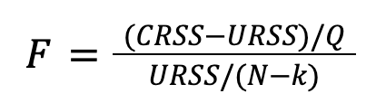
where 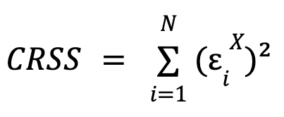 and
and 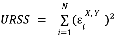 , that is, the sum of the squares of the errors for each model.
 ![]() is the number of constraints imposed on the constrained model (equal to the number of parameters X),
is the number of constraints imposed on the constrained model (equal to the number of parameters X), ![]() the number of values of the time series X for which predictions have been made and
the number of values of the time series X for which predictions have been made and ![]() the total number of parameters to be fitted in the unconstrained model (equal to the sum of the number of parameters β and γ).
the total number of parameters to be fitted in the unconstrained model (equal to the sum of the number of parameters β and γ).
Considering that the mean error can always be set to 0, ![]()
![]() and
and ![]() are proportional to the respective error variances. Intuitively, it can be seen that this magnitude
are proportional to the respective error variances. Intuitively, it can be seen that this magnitude ![]() is the distance between the two variances (moreover, it will always be positive, since by construction
is the distance between the two variances (moreover, it will always be positive, since by construction ![]() ), normalized by “the facility” of the unconstrained model to make more optimal predictions than the constrained one.
), normalized by “the facility” of the unconstrained model to make more optimal predictions than the constrained one.
The latter can be seen in the fact that ![]()
![]() is dividing, which indicates that the fewer free parameters the constrained model has with respect to the unconstrained one, the easier it will be for the latter to make better predictions than the former by construction. Therefore, with the remaining fixed values this “distance” between the two becomes smaller as
is dividing, which indicates that the fewer free parameters the constrained model has with respect to the unconstrained one, the easier it will be for the latter to make better predictions than the former by construction. Therefore, with the remaining fixed values this “distance” between the two becomes smaller as ![]() increases.
increases. ![]() is multiplying, since the greater this difference (or equivalently, the greater the value of the
is multiplying, since the greater this difference (or equivalently, the greater the value of the ![]() ), the difference in the number of parameters to be fitted for each model will be less noticeable and, therefore, they will be on a more equal footing in terms of being able to make accurate predictions.
), the difference in the number of parameters to be fitted for each model will be less noticeable and, therefore, they will be on a more equal footing in terms of being able to make accurate predictions.
The term ![]()
![]() dividing can be understood as a normalization factor to make the magnitude dimensionless.
dividing can be understood as a normalization factor to make the magnitude dimensionless.
The formal way of thinking about this statistical test is that the difference between ![]()
![]() and
and ![]() (normalized by the rest of the factors) follows a distribution of
(normalized by the rest of the factors) follows a distribution of ![]() if the null hypothesis is true.
if the null hypothesis is true.
In order to evaluate the hypotheses, the value of ![]()
![]() in a p-value (because, as mentioned above, this difference follows a certain distribution if the null hypothesis is true). If the value of
in a p-value (because, as mentioned above, this difference follows a certain distribution if the null hypothesis is true). If the value of ![]() is above a certain threshold (equivalent to the p-value below another certain threshold which is usually taken as 0.01), the difference between
is above a certain threshold (equivalent to the p-value below another certain threshold which is usually taken as 0.01), the difference between ![]() and
and ![]() is sufficiently large to consider that the unconstrained model makes better predictions than the constrained model, thus rejecting the null hypothesis, and considering that causality exists (i.e. the result
is sufficiently large to consider that the unconstrained model makes better predictions than the constrained model, thus rejecting the null hypothesis, and considering that causality exists (i.e. the result ![]() is statistically significant). If the result is the opposite, the null hypothesis is accepted and there is no causality.
is statistically significant). If the result is the opposite, the null hypothesis is accepted and there is no causality.
Returning to the parameter we left to fix, ![]()
![]() the first restriction is usually imposed by the physical meaning of the time series, or by being interested in studying a certain lag in particular. In case after this the test is to be performed with a set of lags, the one that generates the most significant causality, in case there is a set of them satisfying the causality condition, is the one that minimizes the p-value or equivalently maximizes
the first restriction is usually imposed by the physical meaning of the time series, or by being interested in studying a certain lag in particular. In case after this the test is to be performed with a set of lags, the one that generates the most significant causality, in case there is a set of them satisfying the causality condition, is the one that minimizes the p-value or equivalently maximizes ![]() .
.
Finally, it is very important to note that in order to be able to apply this methodology we need the errors associated with the predictions, for each of the models, to meet the requirement of following a normal distribution, centred at 0 (here the reason why we mentioned that we could not only take the mean of the errors to 0, but that we would need to do so). In mathematical notation: ![]()
![]() .
.
Advantages and restrictions of Granger causality
Granger causality has a series of disadvantages when it is used to find causalities between time series, which should be mentioned:
- As it is a purely mathematical methodology, it does not allow for an explanation of that causality, since one that occurs as a consequence of cause-effect is indistinguishable, for this algorithm, from one that happens by chance.
- It is not able to distinguish when the behaviour of two time series is determined by a third, distinct time series, from when it is determined between them.
However, it should be noted that these problems and limitations are found in all causality algorithms that work with only two time series at a time. Those that work with more time series at the same time, it is very likely that disadvantage 2 is not present, but the computational cost of these algorithms increases enormously.
Despite this, it performs better than other methods in its class, such as lag regression, where the predictive power of the second time series is not evaluated in the context of also being able to use values from the first.
Conclusion
In this article, we have analyzed the properties of time series that appear when they are related and compared to each other. Thanks to them, we can obtain new relevant information from the data that, if the time series were evaluated individually, would be “hidden”.
If you found this article interesting, we encourage you to visit the Data Science category to see other posts similar to this one and to share it on networks. See you soon!
