Demand forecasting and suitable pricing are two key factors in any business. In the hotel context in particular, and more specifically in the online segment, these tasks are of vital importance due to the dynamic nature of prices and high competitiveness. Automating these processes is key to a quick adaptation, which is why more and more hotels are supporting their decisions in recommendation systems or RMS.
In this article, we present a hotel demand forecasting model and a strategy for choosing the optimal price in order to maximize expected profits. The structure of the article is summarized below.
In section 2 we describe the data set used for this case study. In section 3, we present the demand forecasting model, based on time series. In section 4, we explain how the above prediction is used to generate possible future scenarios through Monte Carlo simulations. In section 5, we will study the effect of price on demand from historical data. These results will be used in section 6 to calculate the optimal price on the simulations generated in section 4. In section 7 we present the results obtained in each of the previous sections. Finally, in section 8 we summarize the work done and suggest further improvements.
The data set we use is a three-year simulation of bookings at a certain hotel, in whose data we have included the effect of weekly and yearly seasonality. We will use the data up to a certain date, the in-sample period, to predict future demand and propose an optimal price over the remaining dates, the forecast period.
It is assumed that the hotel accepts reservations for a specific day of arrival since 𝑇 = 10 days in advance, up until the same day of arrival. The prices are fixed once a day, so at the beginning of each day the hotel manager sets the prices for the current day and the next 𝑇days. These prices are kept during the whole day, so all reservations made on that day are charged these rates. However, the next day, the corresponding 𝑇 + 1 prices are set again, which may be different from those set on the previous day. The hotel capacity is 𝐶 = 100 rooms.
We have detailed information of price and total demand for each day of arrival and each booking day. The dataset also provides the period or season in which each check-in day is included, both for historical data and for the dates to be predicted. In this case there are four distinct periods:
Very Low Season (Very Low): December, January and February.
Low season(Low): March, October and November.
High season(High): April, May and September.
Very High Season(Very High): June, July and August.
Thus, the data set has the following columns:
ReservationDate: the day on which the reservation is made.
CheckInDate: the day of check-in.
ADR: the price set on the day of reservation for that day of check-in, in dollars.
Demand: number of reservations on the reservation date for the check-in date.
Season: the period in which the check-in day is included.
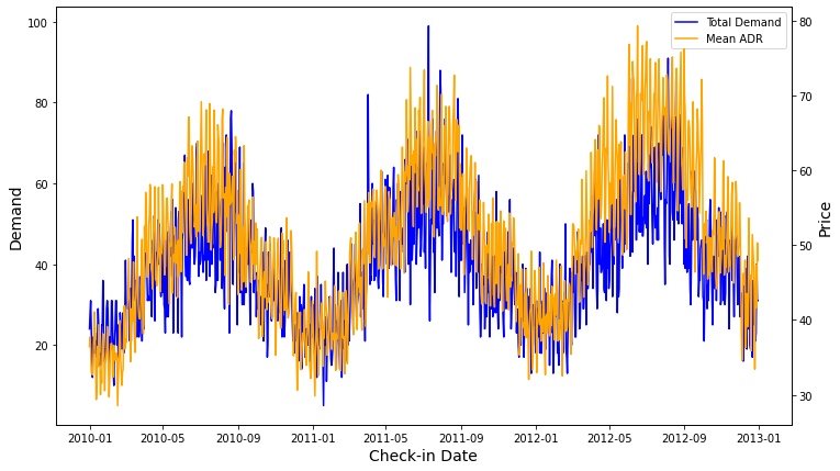
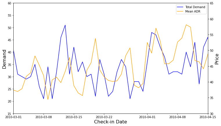
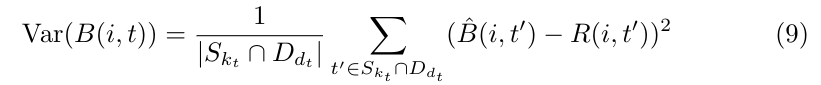
Figure 1. Above, evolution of total demand and average price for each check-in day in our dataset, in which the annual seasonality and the positive correlation between demand and price can be observed. Below, detail of the previous graph, where the weekly seasonality can be appreciated.
Figure 1 shows both aforementioned annual and weekly seasonality, as well as a slight upward trend in both demand and price over time. A strong positive correlation between price and demand is also observed, as is often the case in the hotel industry.
Prediction of future bookings
We now define the process by which we predict future demand. Let 𝑅(𝑖, 𝑡) be the total number of reservations made for a particular check-in day 𝑡, a number of days 𝑖 in advance (difference in days between booking date and check-in date). Note that this number is a realization of the bookings random variable, which we denote by 𝐵(𝑖, 𝑡). We model this random variable as the product of two independent functions as follows.
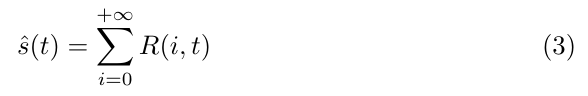
On the one hand, the size of demand according to arrival day, 𝑠(𝑡), represents the total number of expected reservations for a 𝑡 check-in day. On the other hand, the demand shape as a function of advance, 𝐵'(𝑖), represents the fraction of the total number of reservations for a particular arrival day that are made 𝑖 days in advance.
Demand shape
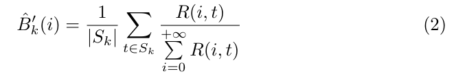
We assume that the demand shape as a function of the booking advance time depends on the season (or period) in which the arrival day 𝑡 is included. As we mentioned in Section 2, there are four seasons in our data, corresponding to periods of very low, low, high or very high activity. Then, for each season 𝑘, we consider the set 𝑆𝑘 of all days falling into that period, and we can estimate the form of demand as a function of anticipation as follows.
That is, for each arrival day of the season under consideration, the fraction of reservations made 𝑖 days in advance is calculated. Finally,the average over all days is computed in order to obtain the demand shape average for period 𝑘. It is assumed that this pattern does not vary in the short term, so the calculated seasonal demand shape will be used in the estimation of future demand.
Demand size
Demand size represents the total expected demand for each check-in day. It is thus estimated from the sample data as the total number of reservations made for each particular stay date.
Remember that our data presents both annual and weekly seasonality. In order to predict the series behavior and thus be able to estimate demand in the future, we deseasonalize it as follows.
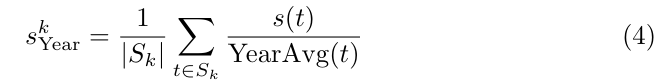
First, we calculate the seasonal index for each season 𝑘, using to the formula
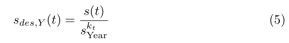
where the denominator represents the average of the series 𝑠(𝑡) in the year which day 𝑡 belongs to. Thus, seasonal index for period 𝑘 is just the average demand for this period, where each value is normalized by its annual average. Then, let 𝑘𝑡 be the period to which day 𝑡 belongs, we calculate the yearly deseasonalized series, as follows
where the subindex 𝑌 represents that this is an intermediate step where yearly seasonality has been removed.
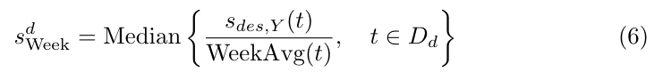
To get rid of weekly seasonality, we follow a similar process. This time, the series 𝑠𝑑𝑒𝑠,𝑌(𝑡) is considered and we use the day of the week 𝑑 instead of the period 𝑘. We also use the median instead of the average to represent the seasonal index of each day of the week. This technique is common in the literature in order to preserve the shape of the weekly peaks. Therefore, we will calculate the seasonal index for day of the week 𝑑 as
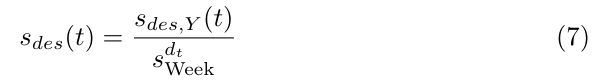
where 𝐷𝑑 represents the set of all days that are of type 𝑑 (e.g. all Mondays). Here, the denominator represents the average of the series 𝑠𝑑𝑒𝑠,𝑌(𝑡) over the week containing day 𝑡. Finally, the deseasonalized series is computed as
where 𝑑𝑡 represents the day of the week of each day 𝑡.
Once we have stripped seasonality out of the series, we forecast it using the Holt-Winters exponential smoothing model, whose parameters are estimated from the sample data. Another option is to use SARIMA models, which require finding the hyperparameters (p, d, q, P, D, Q, m) that best fit the available data. In our case, since we have already deseasonalized the series, we have not found great improvements in the results when using these models. For this reason and due to its relative computational complexity, we use the exponential smoothing approach.
After making the projection of the deseasonalized series, we must undo the previous transformations in order to obtain the total estimated demand for each arrival day. This means that for each day 𝑡 of the forecast period, we must multiply the value of 𝑠𝑑𝑒𝑠,𝑌(𝑡) by their respective seasonal indices and , where 𝑑𝑡 and 𝑘𝑡 are, respectively, the day of the week and the season corresponding to day 𝑡. In this way, we obtain the estimate for the future demand size. The results are shown in section 7.
Demand simulation
Next, we simulate the expected future demand projection assuming that the pricing policy will not change. Thus, the simulated demand is a reference value that will be affected by the pricing policy that is decided to be followed.
We modeled demand as a product of two independent functions, the demand size and the demand shape. For each day in the period to be predicted, we have predicted the demand size ŝ(𝑡) by projecting the deseasonalized series ŝ𝑑𝑒𝑠(𝑡), subsequently multiplying the value by the corresponding seasonality indices. On the other hand, we have obtained an estimate of the form of demand Ḃ𝑘(𝑡) for each period 𝑘 from the historical data. Thus, the expected number of bookings made for a certain arrival day 𝑡 with an advance of 𝑖 days is computed by means of the product
where 𝑘𝑡 is the period in which day 𝑡 is included. In order to simulate the data, we also need to know the variance of the random variable 𝐵(𝑖,𝑡). Since we cannot calculate the variance explicitly, we approximate it from in-sample data as the mean squared error of the bookings variable for all days belonging to the same category, i.e., the same day of the week and the same period, and the same advance 𝑖. Thus, we compute the variance of the booking variable as
where 𝑆𝑘𝑡 is the set of days belonging to the same season 𝑘𝑡 as day 𝑡 and 𝐷𝑑𝑡 the set of days of the same day of the week 𝑑𝑡 as day 𝑡.
From these statistics, we simulate the forward demand for each pair (𝑖, 𝑡) as a normal distribution with average B(𝑖,𝑡) and variance Var( B(𝑖,𝑡)). This distribution is left-truncated at zero, since it is not possible to have negative demand values. Note that the normality assumption could be tested and, if rejected, a different model could be proposed. However, here we have considered enough to control for the average and the degree of dispersion of the demand.
Next, using the Monte Carlo method, we simulate 𝑀 possible demand trajectories for the forecast period. Thus, for each day 𝑡 and each lead time 𝑖 from 0 to 𝑇 (the maximum lead time), we take 𝑀 values from a normal distribution with mean and variance given by equations (8) and (9) respectively.
Estimation of the price – demand relationship
In order to find the optimal price to be set in order to optimize profits, one must take into account the effect that price has on demand. We know that in general the law of demand holds true: a rise in price leads to a fall in demand, and vice versa. However, when studying the data we generally find a positive correlation between price and demand. This is because there are common variables affecting both price and demand, a problem known as price endogeneity. For example, in general we have more potential customers in high season, so hotel managers raise prices, and yet demand is higher than in low season.
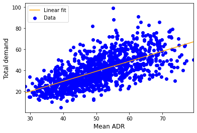
In this context, a simple estimate predicts a positive elasticity value, i.e., that a rise in price causes a rise in demand, contrary to the law of demand. This is shown in Figure 2.
Figure 2. Linear regression of total demand on average price per day of arrival 𝑅² = 0.441. We observe that the slope is positive due to the endogeneity of the price variable.
Therefore, we need to process the data in some way to find the real effect of price on demand, which in particular must be negative. To this end, we proceed as follows.
First, we divide the data into similar subsets, that is, we group together days that belong to the same season and are of the same day of the week. For each subset, we calculate the average of the prices and the number of reservations obtained, which will be the reference prices and demands for that subset. Finally, we normalize the historical prices and demands by dividing each of the prices and demands by its corresponding reference value.
In this way, we hope to isolate the causal effect of varying price on demand. For example, a normalized price greater than 1 means that the price set was higher than the average price under the same conditions (e.g. because the hotel was almost full). Such a choice might result in a lower demand than the average demand under the same conditions, so the normalized demand would be less than 1.
In this case, we consider a linear regression of normalized demand on normalized price for each of the 4 seasonality periods. After fitting each model using the data for each period, we have that
where 𝑝𝑛𝑜𝑟𝑚(𝑖,𝑡) and 𝑑𝑛𝑜𝑟𝑚(𝑖,𝑡) are the normalized price and demand for a certain arrival day 𝑡 and lead time 𝑖, and 𝑘𝑡 is the period to which day 𝑡 belongs.
In the next section, we use this relationship to predict how expected demand will increase or decrease depending on the price we set on each particular day. In this way we can calculate the expected profits for a particular price choice more reliably.
Optimal price calculation
In this section we define the strategy followed to find the optimal price. The objective is to fix the set of prices that maximizes profits in the forecast period, which implies a choice of price for each day 𝑡 and each possible lead time 𝑖.
If we do not impose any restrictions on the behavior that the price should follow, this problem can become extremely complex. In particular, the choice of the optimal price given a certain time in advance 𝑖 depends on the expected profits to be obtained in the forthcoming days, which in turn depend on the price to be set for each of these days. For example, if the hotel is not expected to fill up, the price to be set should be relatively low to ensure a certain occupancy, while the price may be higher if high demand is expected. Such an approach requires solving a recursive problem, for example using dynamic programming.
As we will see in a future post, this calculation can be relatively complex even in simplified situations. To simplify this calculation, we present a parametric model for price based on multipliers.
Dynamic pricing model using multipliers
Let us assume the following approach. The price to be set on each day 𝑡 and each advance 𝑖 could depend on several factors, each of which contributes to setting the final price. In particular, these factors, centered at 1, are interpreted as discounts or premiums that will be multiplied to a reference price. Here, the main assumption of the model lies in the fact that the multipliers are linear with respect to their respective variables, as we will see below. In particular, we take into account two factors: the number of rooms available and the number of days in advance of booking.
Availability multiplier
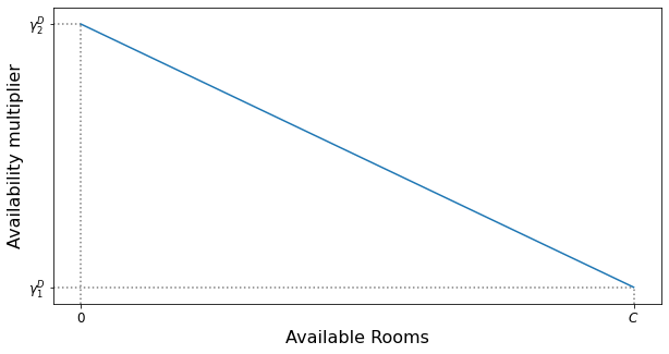
A common practice in the hotel industry is to increase the price as the number of rooms available for the day in question decreases. Thus, in our model the multiplier decreases linearly with the number of rooms available, as seen in Figure 3.
Figure 3. Availability multiplier. Hotel capacity is represented by C.
The multiplier is determined by two parameters. The minimum is given when the hotel is empty and the maximum