BigQuery has become in recent years a powerful tool for data storage and analysis in the cloud. Its size, scalability and all the features it offers would be difficult for a user or company to replicate from scratch due to cost and logistics. In addition, all maintenance and management is handled by Google.
Like any other cloud service, in this case a platform as a service (PaaS), one of the aspects to pay special attention to in order to get the maximum benefit from it will be to know its cost and billing.
During this post we will analyze and give some tips that will help us to have a better control over these costs, as well as to improve the performance of our queries in some cases.
Billing in BigQuery
To begin with, the charges of this platform can come from two different points: firstly, there will be a billing for the storage of the data as such and, on the other hand, for the costs derived from the processing of the data.
Regarding storage, we will be able to opt for different methods. In this case, we will focus on “ON-DEMAND” billing, if we want to make calculations as approximate as possible, Google offers an online calculator that can help us to make an estimate of costs quickly.
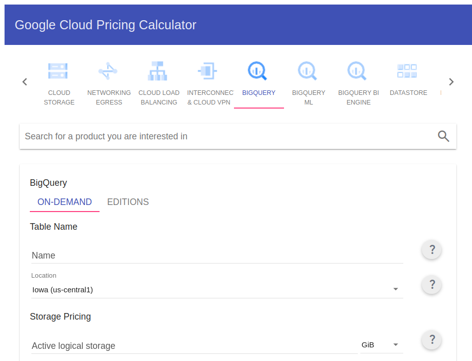
In general terms, these prices range around $20 per TB ($0.025/GB) stored per month.
Generally speaking, the ON-DEMAND price is around $5 per TB processed (the first TB per month is free). And this is where we will focus on some best practices to reduce this amount of data processed during our queries.
During the execution of the queries, the BigQuery interface will inform us of the data to be processed and will be a point to take into account before launching our queries.

Data Exploration
In order to explore our data, on a conventional DB we tend to perform some practices that in BigQuery will not be optimal, especially due to its cost. A clear example is to make queries of the type:
SELECT * FROM `dataset.table_name` LIMIT 10Structurally, BigQuery stores data at the column level, that is, it will process (and bill) only the columns that we select. Therefore, to avoid additional costs, it is advisable to select only what is strictly necessary. Below we can see a comparison:

We should also take into account that BigQuery provides us with data visualization tools that can avoid generating additional costs when exploring the data. For example, if we want to analyze a sample of the data, it will be convenient to use the data preview instead of executing a type statement:
SELECT * FROM `dataset.table_name` LIMIT 10Since in some cases like the one shown below, the total of the table would be processed even though we want a small set of records. Below we can see how the fact of indicating a LIMIT of the records, does not affect the amount of data processed.

This preview is totally free and together with the details or schema tabs, can give us enough information about what the table contains and its characteristics without the need to make queries with an associated cost.
Creation and replication of tables
Another of the tasks that we can perform in our day-to-day work is the transfer of data between tables. Sometimes an exact copy of this data is required as a snapshot or for separate testing, we could think of doing this in the following way:
CREATE OR REPLACE TABLE
 `project_name.data_test_blog.data_mobile_test_no_cluster`
AS
SELECT
 *
FROM
`bigquery-public-data.catalonian_mobile_coverage_eu.mobile_data_2015_2017`
Although this query is perfectly valid, and can fulfill its function, BigQuery allows us to perform this type of operation in various ways depending on our needs, and in many cases, without any associated cost.
One of the most trivial cases that will have the same effect as the query we have just seen is the COPY method. This will allow us not only to copy the content, but also to copy the metadata associated to the table, partitioning, clustering, etc.

In other cases, we can even resort to an even lower cost operation, the cloning of the table. For this, again, a complete copy of the data and metadata of the original table will be made, and there will also be no associated storage cost, at least for those records that remain the same as the original table. This can be interesting when a backup is needed or to perform separate jobs on the same table. Next, we can see an example of how the creation of one of these clones will look like.
CREATE OR REPLACE TABLE
`data_test_blog.data_mobile_test_cluster_CLON` CLONE `data_test_blog.data_mobile_test_cluster`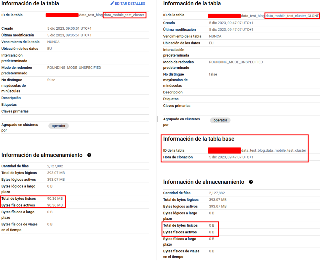
Example of cloned table. The physical storage used is the same as the original table.
Another option available, similar to cloned tables, is to generate snapshots (of some point in the last 7 days) on a base table, again there is no cost associated with the query or storage. These tables have the characteristic of being lighter in terms of processing, but they are immutable.
CREATE SNAPSHOT TABLE
 `data_test_blog.data_mobile_test_cluster_SNAPSHOT` CLONE `data_test_blog.data_mobile_test_cluster` FOR SYSTEM_TIME AS OF TIMESTAMP_SUB(CURRENT_TIMESTAMP(), INTERVAL 1 day)
The use of all these alternatives for data replication should be carefully studied according to the needs of the case, since some of these tables do not behave as conventionally created tables would.
Partitioning and clustering
With regard to the structure of the tables, we must try to make them as easy as possible to interact with, so that the costs are also lower. Two techniques to consider are clustering and partitioning.
Similar to what was mentioned at the beginning of the post regarding the storage by columns, we can indicate when creating the tables if we want them to be partitioned in some way, which means that BigQuery will treat them as separate blocks internally, being these different fragments indexed. This means that if we filter by this field, BigQuery will not need to access the complete data, since it will index directly the required fragment.
Below, we can see the comparison between a table without partitioning and the same partitioned by a date field:

This has its limitations and can only be performed on certain types of columns, usually on fields of type DATE or INTEGER.
The partitioning of these tables also offers us other facilities and cost reduction related to their partitioning. One example is the deletion of partitions:

This type of partition deletion not only has a cost advantage, but also, since that block is stored internally independently, it does not require the rest of the table to be reorganized in any way, as would be necessary if we delete contiguous records.
On the other hand, clustering can be applied to the creation of the tables, which will give us the ability to internally sort the table based on a desired field, that is, the records that have an equal value for the field in which the clustering is performed, will be placed adjacent to each other in the table. This process can be especially useful if we frequently cluster or sort by such a field, as the time and computational cost will be much lower. This is because BigQuery would only access that fragment of the table, since it stores metadata about where those clusters begin and end.
In most occasions, if you want to use this method, it is interesting to do it in conjunction with partitioning.
Below, we can see an example of a table created with a clustering on one of its fields, also this time we will use another of the tools provided by BigQuery after the execution:
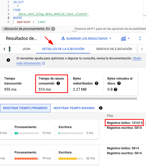
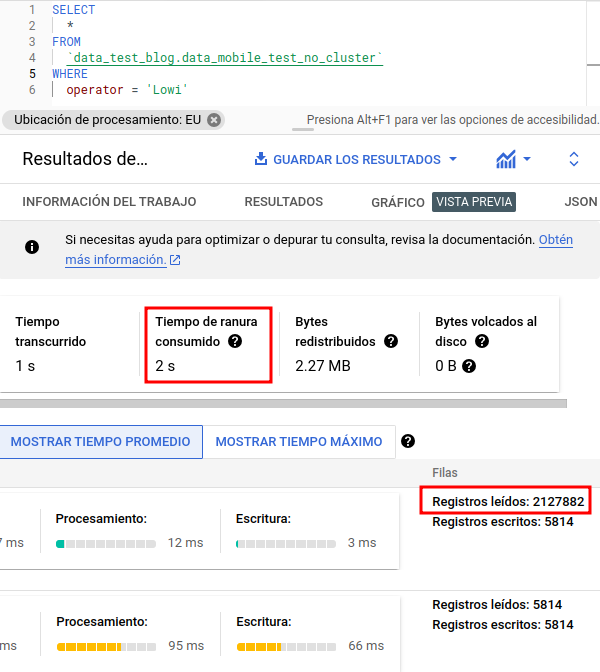
In this case, after executing the script, we have gone to the “Execution details” section which, together with the execution graph, will help us to analyze the behavior of our queries.
We will be able to analyze the consumption of slots (resource assigned by BQ for processing), execution times, records read, etc.
Here we can see that, although the execution time is similar (we are dealing with a small dataset), we can see that the slot consumption time is much higher, as well as the number of records accessed.
Conclusion
Although this type of platforms offers us in a simple way a great set of possibilities, performance and cost, they will only be optimal if we pay attention to all those details that are in our hand. In this post we have seen some of them that if followed can make the difference.
If you found this article interesting, we encourage you to visit the Data Engineering category to see other posts similar to this one and to share it on networks. See you soon!

