Application of Survival Analysis to price changes

In recent years more and more companies are using machine learning and statistics to optimize their business processes. Survival analysis is a little known branch of statistics but it can be useful in many situations. In this post we show some basic concepts of survival analysis and we will see how it can be used in a real business situation.

Basic concepts

Survival analysis studies the time to the occurrence of an event. This time is called event time and is a non-negative random variable that indicates the time between two events of interest. For example, from the application of a treatment to the death of the subject or from the installation of a machine to its failure. It is usually denoted by 𝛵.

If we consider the probability that the time of the event is greater than a certain value, we obtain what is known as the survival curve. Mathematically it is represented as 𝑆(𝑡) and is defined as 𝑆(t) = 𝑃(𝛵>𝑡) =1-𝑃(𝛵𝑡) = 1 – 𝐹(𝑡) where 𝐹(𝑡) is the cumulative probability function.

The hazard function at time 𝑡 represents the probability that the event of interest will occur at the instant immediately following 𝑡. Mathematically it is represented as ℎ(𝑡) and is defined as ℎ(𝑡) = 𝑓(𝑡) / 𝑆(𝑡) donde 𝑓(𝑡) represents the density function of the random variable 𝛵. 

One of the most common characteristics of data from survival analysis studies is truncation or censoring. This occurs when we do not know the exact time at which the event of interest occurs. 

We understand right censoring to exist when we know that the event occurs after a time 𝑡₁ but not exactly when. This type of truncation is common in medical studies, in which participants are followed for a given amount of time and the event does not occur for some of them before the end of the study.

Left censoring occurs when the event is known to occur before a time 𝑡₁ but we do not know exactly when.

A last type of truncation is interval censoring. This occurs when we do not know the exact time of one of the events of interest but we know that it occurs between two instants 𝑡₁ and 𝑡₂ . A special type of interval censoring is double interval censoring, which occurs when we have an interval for each of the events of interest.

The following figure shows graphically each type of censoring.

Why not linear or logistic regression?

The presence of observations with some type of censoring is what makes the use of traditional regression methods impossible in many cases. However, even in the absence of censoring, survival analysis is preferable for two other reasons:

1. The time of the event is a random variable that is biased in addition to being restricted to the positive real number which does not fit with the distributions used in linear regression models.
2. In many cases the objective is not to understand the mean time to event but the shape of the survival curve or hazard function.

Airline ticket price changes

In websites such as Skyscanner, Kayak, or Edreams, users usually consult a flight several times before deciding to buy it. For each of these queries, the site must make a request to the provider, which can increase the operational cost as well as saturate the provider’s server. In response to this problem, many portals create a database with the flights and prices that have been recently consulted and only request the supplier when the user is about to buy. This database is commonly known as a cache memory.

A cache memory has its own pitfalls as storing data also comes at a cost to the company. Ideally, the optimal strategy is to store only those flights that will be consulted again in the future and to do so as long as the stored ticket price has not changed.

The second problem is the one that concerns us in this post. That is, given a set of cached ticket prices, how long should we keep them in memory in order to minimize costs as well as the difference between the displayed price and the final price at which the customer buys?

This question remains complex because it must take into account costs that are variable over time such as the monetary costs incurred in storage and the subjective cost of providing a wrong price to the user. However, we can simplify the question to one whose answer provides useful information no matter what the costs are. So what is the probability that the price of a ticket is still valid given the number of days we have had it stored in memory?

By answering this question we can provide the company with information that can be used to subsequently establish subjective thresholds, such as only keeping a price in the cache if and only if the probability of it remaining in force is greater than 80%.

To use survival analysis in this case, we assume that price change is the event of interest and each price/ticket is an individual that is born, lives for a while and dies. Since these portals have multiple providers and flight types we opt for a parametric model so that different survival curves are indirectly estimated. Specifically, the AFT with Weibull distribution will be used, which models the logarithm of the time of the event and produces a survival curve given by a simple function:

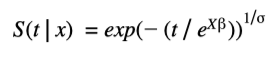
Where 𝑘 and λ are the shape and scale parameters of a Weibull distribution and 𝛽 is the vector with the influence of the χ explanatory variables.

Due to the volume of data handled by these flight portals, PySpark may in many cases be the only option for training the model using all the data (see the Apache Spark documentation) 

The data provided by the company are requests made to suppliers that show us the characteristics of the flight, the date when the request was made and the price obtained:

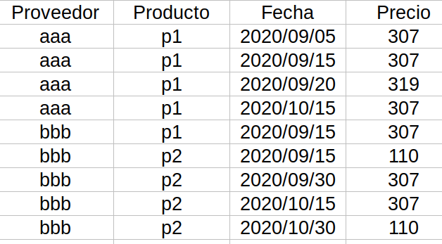
In our case the product is defined by 4 variables (there are also some variables that are parameters passed to the supplier but are of no relevance other than defining the product and are therefore not mentioned): the date of the flight, the type of flight (business, regular), the city of origin, the destination and the other flights included in the request (this variable is included since a flight could have several stopovers and airlines may offer a discount if all sections of the trip are purchased with the same company).

Before fitting the model, these data must be preprocessed so that they are in a format suitable for the model. The goal of the preprocessing is to bring the data to a state where each row is a price along with the duration of the price, which makes it possible to use the AFT model.
In addition, the PySpark implementation of the AFT accepts data only with right censoring so data with other types of censoring must be brought into this form. 

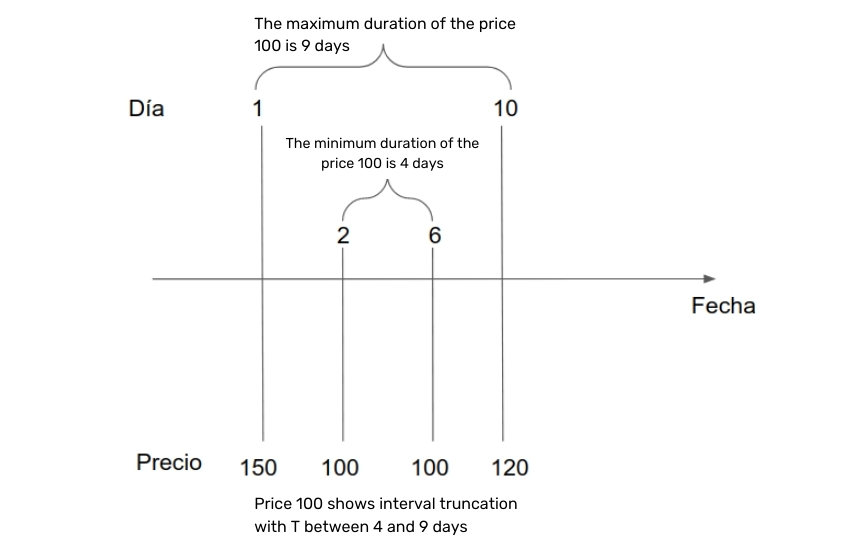
Since we only observe prices at a few instants in time, if we assume that there are no other price changes between our observations, each of the prices in our data is an observation with double interval censoring. For example, the following figure depicts each of the times we have obtained a price for a certain flight during a certain period. The price 100 that we observed on days 2 and 6 could have started at most on day 1 since we obtained a different price on that day. Also, the last day it could have been in effect is day 10, so we know that the time span of this price is 4 to 9 days.

Applying this reasoning to the example data of the previous section, we obtain a table as follows:

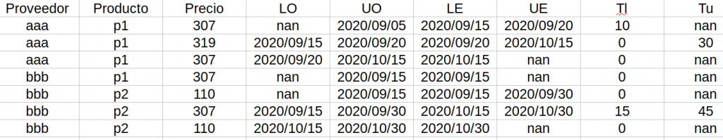
The next step is to use the interval [𝛵𝜄, 𝛵𝑢] of the variable𝛵 to obtain a single price duration time with which to feed the model. In the literature it is common to use the midpoint of the interval to obtain a single duration variable, so we apply this method to observations that have all time bounds defined. For those with right censoring, we add a variable indicating that this truncation exists. The observations with lower limit equal to zero do not give us relevant information since it is the whole interval of the duration variable so we discard these observations. The final table that we will use to train the model has the following form:

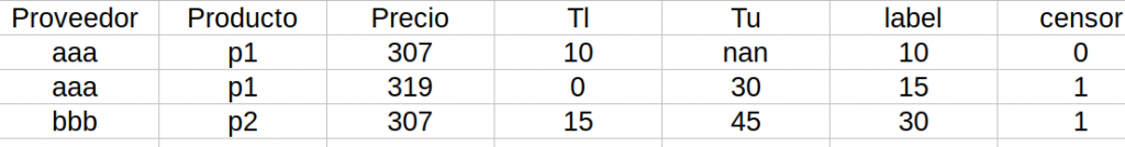
An important fact worth emphasizing is that for PySpark’s AFT implementation the variable indicating censoring “censor” has the value zero when the observation is right censored and one when it is not.

With this table we can create the model in Spark. Note that in PySpark it is not possible to obtain the survival curve from a trained AFT model. However, it is possible to provide the model with a vector of quantiles that we want from the survival curve. For example, if we estimate the model with a vector whose only element is 0.5 then when making predictions, in addition to the average time, it is possible to obtain the day on which the survival probability reaches that value. To approximate the entire survival curve we can then use a function that interpolates between the quantiles with which we have trained the model.

The code to train the model with the simulated data we have been using is:

import org.apache.spark.ml.linalg.Vectors
import org.apache.spark.ml.regression.AFTSurvivalRegression

# Label = tiempo que el precio de un boleto es válido
# vectors = variables explicativas = ['tiempo hasta que salga el vuelo', 'el vuelo es business'] 
training = spark.createDataFrame([
    (10, 0.0, Vectors.dense(50, 0)),
    (15, 1.0, Vectors.dense(180, 0)),
    (30, 1.0, Vectors.dense(200, 1)),
    (12, 1.0, Vectors.dense(60, 0)),
    (20, 0.0, Vectors.dense(45, 1))], ["label", "censor", "features"])
quantileProbabilities = [0.3, 0.6]
aft = AFTSurvivalRegression(quantileProbabilities=quantileProbabilities,
                            quantilesCol="quantiles")

model = aft.fit(training)

# Imprimimos coeficientes
print("Coefficients: " + str(model.coefficients))
print("Intercept: " + str(model.intercept))
print("Scale: " + str(model.scale))

# Hacemos predicciones sobre los datos de entrenamiento
# Aquí nos devuelve una columna con los tiempos en los que se alcanza 
# una probabilidad de supervivencia igual a 0.3 y 0.6 (colocadas en quantileProbabilities) 
model.transform(training).show(truncate=False)

Conclusion

In this post we have seen basic concepts of survival analysis and we have demonstrated the whole process to transform business data into data that fit the AFT model implemented in PySpark. The main idea is that by reading these lines you will consider using this tool as an additional way to solve the problems faced by certain companies.

If you found this post useful, we encourage you to see more articles like this one in the Data Analytics category in our blog and to share it with your contacts so they can also read it and give their opinion. See you in networks!