What are Vehicle Routing optimization Problems?
The concept of Vehicle Routing Problem (VRP) is a generalization of the well-known Traveling Salesman Problem (TSP). Specifically, the VRP is a pure optimization problem whose objective is to determine the most efficient route. Therefore, it seeks to have a fleet of vehicles deliver goods or services while minimizing costs as much as possible.
Basically, in TSP, there is a map of a city with multiple points that an individual must visit to return to their point of origin, taking the shortest possible route. In contrast, the VRP is not limited to just one person. In fact, there may be N individuals who normally have to deliver items to various points in the city. This makes the problem more complex than the TSP.
In this article, we will look at different variants of this problem and how to approach these variations in order to implement them in the solver of our choice. To do this, we will use Google OR-Tools as an example.
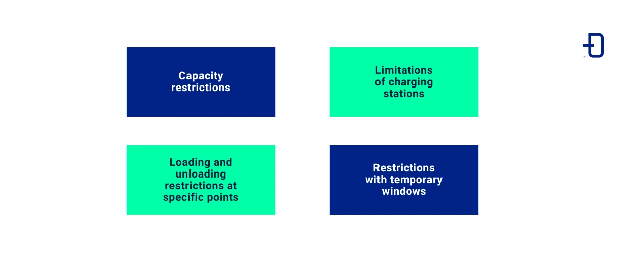
Vehicle Routing Problem: Variants
Capacitated Vehicle Routing Problem
The Capacitated Vehicle Routing Problem (CVRP) is a variant of the VRP that introduces a constraint whereby each vehicle has a limited load capacity that cannot be exceeded.
In this most basic formulation of the VRP, we have N vehicles, X cities, and we want to minimize the total distance traveled. In addition, it is typical to add one more limitation, which is that each of the X cities must be supplied with a quantity of supplies that we will call Xs. In turn, this is included in the context that each of the N vehicles has a maximum capacity of supplies that it can carry, which we will call Ns. Ultimately, the problem becomes more realistic by introducing this constraint.
VRP with charging stations
Vehicle Routing Problem with Charging Stations (VRP-CR) is a variant of VRP focused on vehicle route planning. In this case, it takes into account the points where the vehicle can recharge.
To do this, we simply add new nodes where we want to be able to recharge. Next, we will give these nodes a negative demand equal to the largest capacity of our vehicles. Then, we will add an equally large slack and the restriction that no vehicle can carry negative capacity.
This way, there could be a vehicle that is able to recharge with goods during its trip, which would allow for its reuse. Otherwise, a vehicle could only carry, at most, its capacity.
def add_capacity_constraints(routing, manager, data, demand_evaluator_index):
    """Adds capacity constraint"""
    vehicle_capacities = data["vehicle_capacities"]
    capacity = 'Capacity'
    routing.AddDimensionWithVehicleCapacity(
        demand_evaluator_index,
        30, # Slack equal to max possible load, so reloads can occur
        vehicle_capacities,
        True,  # start cumul to zero
        capacity)
    capacity_dimension = routing.GetDimensionOrDie(capacity)
    for v in range(manager.GetNumberOfVehicles()):
        end = routing.End(v)
        capacity_dimension.SetCumulVarSoftUpperBound(end, 0, 100_000) # End route empty
    # Allow dropping reloading nodes with zero cost.
    for node in [1]:
        node_index = manager.NodeToIndex(node)
        routing.AddDisjunction([node_index], 0)
VRP with loading and unloading at specific points
In this variant, we must add the restriction between point A (where we want to start) and point B (where we want to arrive), that the distance traveled by the vehicle is strictly less at A than at B, and also that it visits both nodes. With this formulation, it is also possible to leave cargo at the visited node without modifying the restrictions. Thus, it is possible to indicate that 5 objects are picked up at A but another 5 are left at B.
In this way, we can force the movement of specific objects from node A to node B. This can be important in cases where certain items are only present at one node and are ordered by another.
def add_pickup_dropoff(routing, manager, data):
    # Define Transportation Requests.
    for request in data["pickups_deliveries"]:
        pickup_index = manager.NodeToIndex(request[0])
        delivery_index = manager.NodeToIndex(request[1])
        routing.AddPickupAndDelivery(pickup_index, delivery_index)
        routing.solver().Add(routing.VehicleVar(pickup_index) == routing.VehicleVar(delivery_index))
        distance_dimension = routing.GetDimensionOrDie('Distance')
        routing.solver().Add(distance_dimension.CumulVar(pickup_index)
            <= distance_dimension.CumulVar(delivery_index))
Vehicle Routing Problem with time windows
This formulation focuses on limiting when a city can be visited within a valid time interval. To achieve this, it is necessary to add a new dimension, the time dimension, which measures the interval each vehicle is in at the time of travel. With this dimension, we only have to add the restriction that if a city is visited, it must be within the specified time window.
In this way, we can add the restriction that only one node can be served during certain times. This is very useful when, for example, a product needs to arrive before a certain time to be processed or served.
def add_time_window_constraints(routing, manager, data, time_evaluator):
    """Add Time windows constraint"""
    time = 'Time'
    max_time = data['vehicle_max_time']
    routing.AddDimension(
        time_evaluator,
        max_time,  # Alow waiting time ( vehicles can idle )
        max_time,  # Maximum time per vehicle
        False,
        time)
    time_dimension = routing.GetDimensionOrDie(time)
    # Add time window constraints for each location except depot
    for location_idx, time_window in enumerate(data['time_windows']):
        if location_idx == 0:
            continue
        index = manager.NodeToIndex(location_idx)
        time_dimension.CumulVar(index).SetRange(time_window[0], time_window[1])
        routing.AddToAssignment(time_dimension.SlackVar(index))
    # Add time window constraints for each vehicle start node
    for vehicle_id in range(data['num_vehicles']):
        index = routing.Start(vehicle_id)
        time_dimension.CumulVar(index).SetRange(data['time_windows'][0][0],
                                                data['time_windows'][0][1])
        routing.AddToAssignment(time_dimension.SlackVar(index))
Example with all restrictions
To illustrate a problem that applies all the formulations mentioned above, we implement a model that includes all these restrictions.
This model consists of a fleet of vehicles that have to transport people from different starting points to different destinations during one day. In addition, they have a maximum allowed waiting time.
As for the data for this example, we created a small synthetic dataset. In it, there are five hotels and one airport that have different needs for moving people at certain times between those two points.
Distance and travel time matrix
Below, we see the distance matrix between all locations:
| PortBlue Club Pollentia Resort & Spa | EIX Lagotel Holiday Resort | Universal Hotel Lido Park & Spa | MLL Mediterranean Bay | AHOI! Urban Beach | Airport | |
| PortBlue Club Pollentia Resort & Spa | 0 | 13 | 76 | 66 | 64 | 60 |
| EIX Lagotel Holiday Resort | 9 | 0 | 77 | 66 | 65 | 60 |
| Universal Hotel Lido Park & Spa | 72 | 77 | 0 | 38 | 37 | 32 |
| MLL Mediterranean Bay | 68 | 70 | 38 | 0 | 1 | 11 |
| AHOI! Urban Beach | 67 | 68 | 37 | 1 | 0 | 9 |
| Airport | 60 | 62 | 31 | 7 | 6 | 0 |
This would be the travel time matrix between all locations:
| PortBlue Club Pollentia Resort & Spa | EIX Lagotel Holiday Resort | Universal Hotel Lido Park & Spa | MLL Mediterranean Bay | AHOI! Urban Beach | Airport | |
| PortBlue Club Pollentia Resort & Spa | 0 | 10 | 63 | 49 | 49 | 43 |
| EIX Lagotel Holiday Resort | 12 | 0 | 63 | 51 | 50 | 44 |
| Universal Hotel Lido Park & Spa | 53 | 56 | 0 | 31 | 30 | 25 |
| MLL Mediterranean Bay | 50 | 53 | 43 | 0 | 5 | 12 |
| AHOI! Urban Beach | 50 | 53 | 43 | 6 | 0 | 12 |
| Airport | 42 | 44 | 34 | 8 | 8 | 0 |
Time constraints
In terms of time constraints, we have a group of people who can be picked up up to 30 minutes after arrival time and who can arrive no later than 60 minutes after arrival. In this case, the orders are as follows:
| Arrival time | Individuals | Origin | Destination |
| 0 | 10 | Airport | PortBlue Club Pollentia Resort & Spa |
| 20 | 20 | Airport | EIX Lagotel Holiday Resort |
| 70 | 10 | PortBlue Club Pollentia Resort & Spa | EIX Lagotel Holiday Resort |
| 70 | 10 | EIX Lagotel Holiday Resort | Airport |
| 70 | 20 | EIX Lagotel Holiday Resort | Airport |
| 60 | 10 | Airport | Universal Hotel Lido Park & Spa |
| 120 | 10 | Airport | MLL Mediterranean Bay |
| 130 | 10 | Airport | AHOI! Urban Beach |
In addition, we have three vehicles available in the model. One of them has a capacity of 10 people and the other two have space for 30.
Example route
Applying all of the above restrictions, we generate this example route:
Objective: 13637
dropped orders: []
dropped reload stations: []
Route for vehicle 0:
 Aeropuerto with demand: 0 Vehicle Load(0) Time(0,0) ->
 Aeropuerto with demand: 20 Vehicle Load(0) Time(20,36) ->
 EIX Lagotel Holiday Resort with demand: 10 Vehicle Load(20) Time(70,80) ->
 EIX Lagotel Holiday Resort with demand: -20 Vehicle Load(30) Time(70,80) ->
 EIX Lagotel Holiday Resort with demand: 20 Vehicle Load(10) Time(70,86) ->
 Aeropuerto with demand: -10 Vehicle Load(30) Time(114,130) ->
 Aeropuerto with demand: -20 Vehicle Load(20) Time(114,130) ->
 Aeropuerto Load(0) Time(114,1500)
Distance of the route: 124km
Load of the route: 0
Time of the route: 114min

Route for vehicle 1:
 Aeropuerto with demand: 0 Vehicle Load(0) Time(0,0) ->
 Aeropuerto with demand: 10 Vehicle Load(0) Time(0,18) ->
 PortBlue Club Pollentia Resort & Spa with demand: -10 Vehicle Load(10) Time(42,60) ->
 PortBlue Club Pollentia Resort & Spa with demand: 10 Vehicle Load(0) Time(70,100) ->
 EIX Lagotel Holiday Resort with demand: -10 Vehicle Load(10) Time(80,130) ->
 Aeropuerto Load(0) Time(124,1500)
Distance of the route: 133km
Load of the route: 0
Time of the route: 124min

Route for vehicle 2:
 Aeropuerto with demand: 0 Vehicle Load(0) Time(0,0) ->
 Aeropuerto with demand: 10 Vehicle Load(0) Time(60,86) ->
 Aeropuerto with demand: 0 Vehicle Load(10) Time(60,86) ->
 Universal Hotel Lido Park & Spa with demand: -10 Vehicle Load(10) Time(94,120) ->
 Aeropuerto with demand: 10 Vehicle Load(0) Time(130,150) ->
 Aeropuerto with demand: 10 Vehicle Load(10) Time(130,150) ->
 MLL Mediterranean Bay with demand: -10 Vehicle Load(20) Time(138,180) ->
 AHOI! Urban Beach with demand: -10 Vehicle Load(10) Time(143,190) ->
 Aeropuerto Load(0) Time(155,1500)
Distance of the route: 80km
Load of the route: 0
Time of the route: 155min

Total Distance of all routes: 337km
Total Load of all routes: 0
Total Time of all routes: 393min
Conclusion
As we have seen, it is possible to alter the constraints of the Vehicle Routing Problem to cover more specific problems. In conclusion, playing with the limitations of the model allows the VRP to be adapted to different real-world scenarios. However, it is sometimes necessary to approach it indirectly due to the nature of how these constraints are expressed. In addition, in this article we have also generated a simple problem where the cases analyzed occur.
If you liked this post, we encourage you to visit the Algorithms category to see other articles similar to this one and to share it on social media. See you soon!
