
The ability to collect and process large amounts of data represents additional value for many companies in today’s market. In the world of sports, baseball was among the first to embrace this shift with the emergence of SABRmetrics in the 1980s. From there, it extended to motor racing and, more recently, to sports such as basketball and soccer. Creating models and metrics through artificial intelligence enables sports fans to analyze the game from a new perspective and allows professionals to gain a competitive advantage over their rivals.
In the case of soccer, probably the most popular metric is the one known as expected goal (xG). The xG is intended to measure the probability that a shot will result in a goal, taking into account variables such as the position of the shot, the position of the goalkeeper or the part of the body with which the shot is taken. As it is a probability, it should take values between 0 and 1, so that for the clearest opportunities (for example, a shot inside the small area without a goalkeeper) it takes values close to 1, and for shots further away or with greater difficulty it tends to 0.
This metric is very useful for coaching staffs and scouting teams to evaluate the finishing or chance-creating ability of different players. So, for example, if we look at the difference between the number of goals a player has scored and the sum of the xG of the shots he has taken, a positive or negative difference will indicate, respectively, a high or low finishing ability of the player. Similarly, if a player’s passes result in high xG shots, this indicates that he is capable of creating clear scoring chances.
Each user generates his xG model based on the available information that he considers most relevant, seeking to match the probability issued as closely as possible to the shot history that he has.
The present study is based on data from Wyscout, one of the largest providers of soccer data, which collects information on all events occurring in each match. A dataset of about 8,500,000 event records is available, containing variables such as the league or match in question, the player involved, the type of event (shot, pass, steal, etc.) or its position on the field, among others. Of these, some 117,000 records are shots, and these are the ones on which our xG model will focus. These events correspond to 25 professional club competitions in Europe and America (national leagues and Copa Libertadores), mostly from the 2020/21 edition (2021 in LATAM and USA).
Preliminary considerations
- The xG metric is intended to evaluate the dangerousness of a shot at the time immediately prior to the execution of that shot. Therefore, information that is subsequent to the execution of the shot, such as whether the shot was blocked or whether the goalkeeper was beaten to the side, cannot be introduced into the model. In this way, the value returned as the a priori probability that such action ends in a goal.
- The xG is intended, among others, to be able to assess the ability of players to create scoring chances (passers), convert them (finishers) or avoid them (defenders). As such, this value should reflect the generic probability that under certain fixed conditions a shot will result in a goal, and therefore be abstracted from specific conditions such as the attacking and defending teams, the players involved or their demarcations, as well as the league, the date or the place where it occurs.
- Each action in the match is tagged with a series of ratings by Wyscout analysts. These represent more or less subjective information, such as whether the pass preceding the shot is a filtered pass, or whether the action constitutes a scoring opportunity. We assume that when using the model, as well as during training, the end user will have access to this information. Let us note that, under the assumption that the labeling follows a uniform and unbiased criterion (for example, that whether a shot is labeled as a clear chance or not does not depend on the player who is shooting), this information does not contradict the generality principle mentioned above, since two identical actions performed by two different players will have exactly the same set of input variables and, therefore, the same value of xG. Therefore, we also introduce subjective variables in our model, as Wyscout does in his own model of xG.
Work development
Let us note that what we want to predict is whether or not a shot will be a goal, so we are faced with a binary classification problem.
To begin with, we perform an exploratory analysis of the available data in which we study the data, the unexpected values and perform variable engineering to enrich our dataset.
Secondly, we will proceed to perform a selection of variables based on different criteria, and on each of these datasets we will fit different supervised models. Then, we will compare their results in order to find the optimal model and its hyperparameter combination for the classification task.
Finally, we will evaluate the best model on a previously unseen dataset to test its generalizability, using as a benchmark the own xG value calculated by Wyscout, which it provides together with the event dataset.
Exploratory data analysis
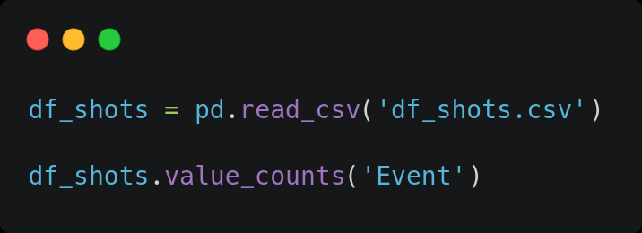
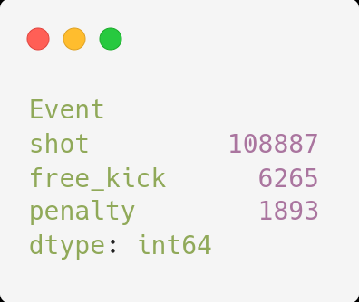
In this phase, we analyze the data and perform the necessary preprocessing. To begin with, we see that our initial dataset contains events of type ‘penalty’, ‘free_kick’ or ‘shot’.
It is usual when performing xG models to discard penalty kicks since they are very isolated actions of the game and with very particular conditions. Therefore, we trained our model only with the records of free kicks and shots in play. After this filter, we have 115,152 shot records.
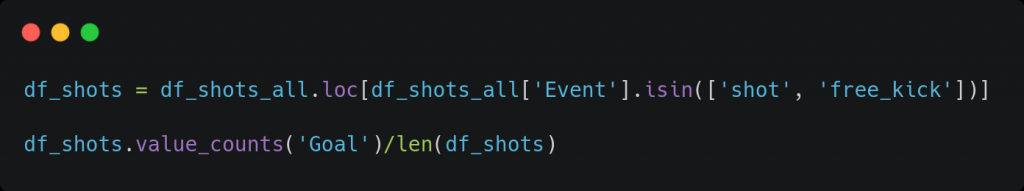
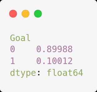
Also, we see that the classes we want to predict (‘Goal’ or ‘Failure’) are very unbalanced, with a ratio of approximately 1 goal for every 9 failures. At this point, we could consider methods to balance the classes, such as using data augmentation or reducing the number of records in the ‘Failure’ class. However, we believe that the first one is dangerous as we have observed that a small modification in a parameter can be differential for the outcome of the shot. On the other hand, the second option would imply reducing the volume of the dataset to about 20,000 records, which we consider too low a number to train a classification model.
On the other hand, the variables that refer to the type of ball possession (counterattack, set piece, etc.) or the type of sub-event (recovery after pressure, key pass, etc.), both for the current and previous events, contain a list of values, so we create a binary variable for each possible value and indicate with a 0 or a 1 if each event contains it (note that each row can have more than one 1, so it is not a one-hot encoding).
In some cases these values are subjective since they have been labeled by a human (e.g., “filtered pass” for the previous event or “goal chance” for the shot), but as we discussed in the Initial Considerations section, we decided to use them anyway.
Continuing with this section, we then discard all the variables that cannot be determined at the moment of the shot, since it is then when the xG must be calculated. Thus, for example, we do not introduce in the model whether it is a blocked shot or whether it is on target. Similarly, context-specific variables, such as the demarcation, the team or league in which the shooter plays, or metrics on the goalkeeper, are discarded. As explained, although it could improve the current model in terms of predictive ability, the result obtained with such variables could not be interpreted as an xG.
The next phase of the process is variable engineering. To begin with, null or outliers (such as a negative distance) are removed and replaced by the mean of the numerical variable in question so as not to introduce bias into the model. Likewise, we retrieved diverse information that may be useful for the classification task, such as the 3 events immediately prior to the shooting event, from which we collected their position on the field, the type of event (duel, pass, throw-in, etc.) or how many seconds before the shot occurred, among other variables.
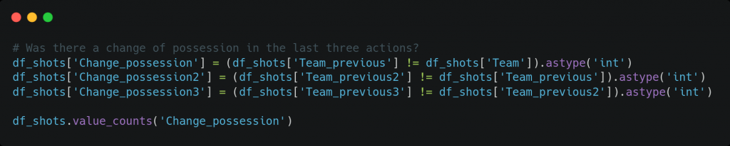
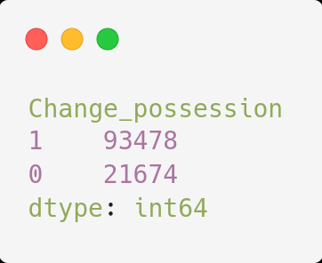
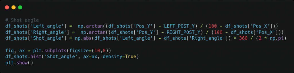
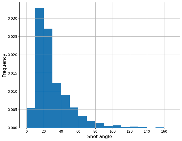
Next, new variables were created from the existing ones. For example, the position (X,Y) of the shot (both normalized between 0 and 100) was replaced by the distance to the center of the goal or the angle of the shot, as these were considered more significant. Likewise, it was calculated whether a change of possession occurred in the three immediately preceding actions.
Finally, one hot encoding of the categorical variables was performed, such as the part of the body with which the shot is taken (right leg, left leg, or other) or the type of event, both current (a free kick or in play) and previous (duel, pass, save, etc.).
Variable selection
After the previous phase, we had 309 variables, many of them binary. As this is a very large number considering the number of records available, it was decided to use only a subset of these to train the predictive models. Different methods were considered for the selection of variables.
- Variables specified in the documentation of the WyScout xG model itself. Since not all variables used are specified, other variables widely used in other xG models were added, with a total of 15 variables.
- Variables with a linear correlation with respect to the dependent variable above a threshold of 0.1 (in absolute value), with a total of 27 variables.
- Variables selected using the Boruta method. This method consists of running a set of N random forests on the union of the set of original variables and a set of shadow variables, consisting of the random permutation of the values of the original variables. Finally, only those variables are selected whose Gini index, or explanatory power over the dependent variable, is above a certain pre-set percentile with respect to the shadow variables. In this way, we keep the significant variables and discard the variables that do not provide valuable information for the classification.
In this case, we have used N=100 random forests, each with T=413 trees (number of trees automatically chosen from the length of the dataset) with a maximum depth of 5, and we use the 100th percentile (we keep only the variables that exceed in explanatory power all the randomized versions). We are thus left with 79 variables.
Data preparation
We next divided the data set into train and test, with a ratio of 80% and 20% and using stratification with respect to the target variable, that is, preserving the proportion of goals and misses in both sets in order to be able to correctly evaluate the model. The test set will not be used during training or model selection, as it represents a data set for which no input is available, and will simply be used to evaluate the generalizability of the final model on an unseen data set.
Subsequently, we perform a standard scaling (between 0 and 1) for any non-binary independent variable, such as the angle of the shot or the time elapsed since the previous action.
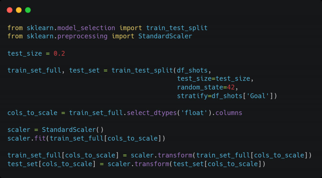
Note that the same scaling is performed for both the training set and the test set, to avoid that the particular characteristics of the dataset may alter the decision of the model. In particular, we scale all data based on the mean and standard deviation of the training set, since the test set represents data not known a priori.
Training and comparison of models
Finally, we proceed to the development of different classification models, using the scikit-learn and keras libraries, among others. Each of these models will be trained and evaluated on each subset of variables previously selected to find the best combination. Also, a grid search will be performed to try to refine the hyperparameters of the model in each case. Both during training (grid search) and model evaluation using the best combination of hyperparameters, 10-iteration cross-validation is used with a fixed seed and again with stratification, in order to evaluate all models under the same conditions.
The models that have been considered and some of the hyperparameters that have been optimized in the corresponding grid search are the following.
- Logistic regression: regularization form (L1, L2), regularization parameter, optimization algorithm.
- Random forest: number of trees, number of variables at each node, maximum depth of trees, etc.
- XGBoost: learning ratio, maximum depth of trees, relative weight of positive class (for unbalanced data sets), etc.
- Neural network (multilayer perceptron): dropout ratio, structures with different number of layers and neurons per layer, activation function in the hidden layers (the logistic function is always used in the output layer), optimization algorithm, etc.
To prevent overfitting, in the XGBoost case, we stop training when, after adding 10 trees, the loss function over the validation set does not decrease. In the neural network, we stop training when the loss function over the validation set increases in two consecutive epochs. In both cases we use as loss function the binary cross-entropy.
The metric chosen to compare the models is the area under the ROC curve (ROC-AUC), commonly used in binary classification problems when there is imbalance in the classes, as in our case. Thus, we will look for the model and the combination of hyperparameters that results in a higher ROC-AUC value. The probability output by this model will finally be our value of xG.
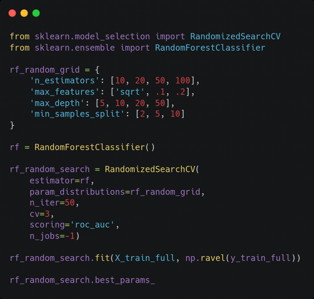
Due to the large number of parameters and the wide range of values to be studied, we divide the grid search into two steps. In the first step, a search is performed within a wide grid of values for each hyperparameter, with the objective of obtaining the optimal order of magnitude of each one. For this case, to reduce training time, we test only a fraction of all possible combinations using the RandomizedSearchCV function of scikit-learn.

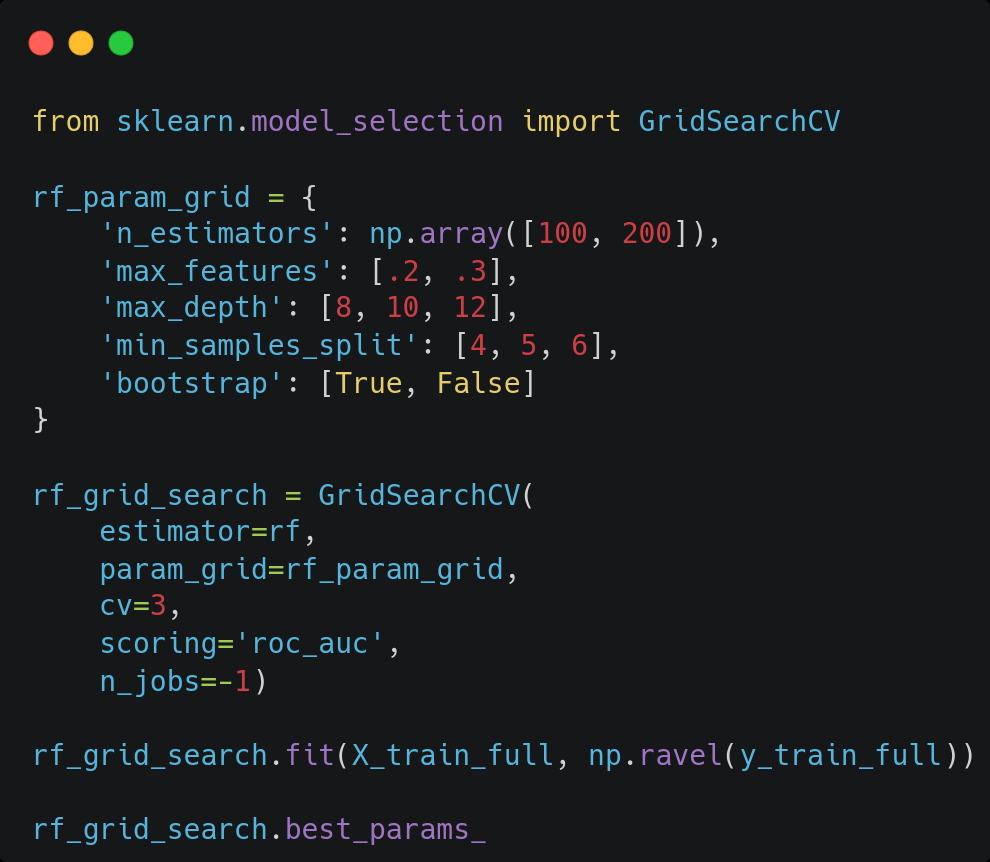
In the second step, we perform a search in a narrower space where we expect to find the optimum. Thus, if the best value for a certain hyperparameter found in the first step was given for a non-extreme value of the considered interval, we set a reduced range centered on that value. On the other hand, if it was given for a maximum (or minimum) of the considered interval, the search is expanded to values larger (or smaller) than that value. This time we use the GridSearchCV function to test all possible combinations, having reduced the search space.
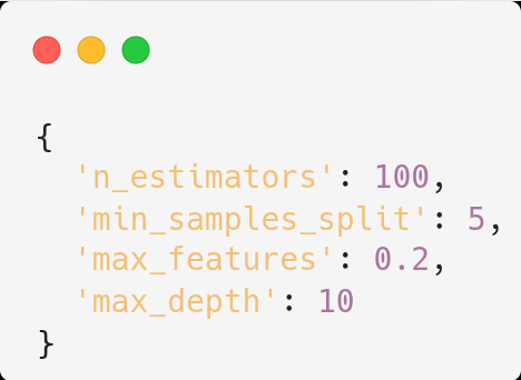
Then, we evaluated the model on the training set using the best combination of hyperparameters found.
In the model evaluation, we set the seed to perform cross-validation, so that all models are trained and evaluated on the same training/validation subsets and thus avoid that the specific choice of these favors one or another model. This is the function for model evaluation for scikit-learn models.
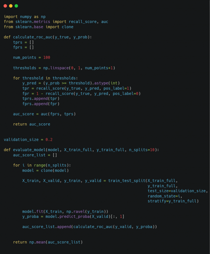
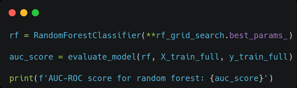
So we evaluate the model with the best combination of hyperparameters found above.
Finally, we compared the metrics obtained for each of the models. The results obtained are shown in Figure 1.
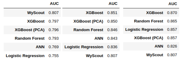
Figure 1. ROC-AUC value obtained with each model and each set of variables (the Wyscout model is included for comparison). From left to right: variables available from the Wyscout model, variables chosen according to linear correlation with a minimum absolute value of 0.1 and variables selected by the Boruta method using 100 random forests and the 100th percentile.
As we can see, the best model obtained in terms of ROC-AUC value has been the XGBoost model in all cases. Let us note that it has improved even to a model a priori more complex as the neural network, probably due to the relatively small size of our dataset. In particular, the best result has been obtained when using the variables selected by Boruta’s method.
Once the best model and the best set of input variables were fixed, we tried to improve the model results by applying principal component analysis (PCA) to our data. This method allows not only to reduce the dimensionality and therefore accelerate the learning process of the models, but it can also favor their performance by eliminating the possible noise or redundancy of the different variables. Therefore, we perform a new grid search on a pipeline in which we apply PCA with different numbers of components and, for each case, we search for the combination of XGBoost hyperparameters that best fits this dataset.
Finally, we choose the best combination of number of principal components and hyperparameters of the model, and re-evaluate it. We compare the metrics obtained with those obtained before performing PCA to determine if they improve the results. In this case, as seen in Figure 1, the model performance in terms of ROC-AUC does not increase when using PCA. This result implies that the gain from removing noise and redundancy by reducing dimensionality does not compensate for the loss of intrinsic information in the process.
Note that different combinations of number of principal components, model type and model-specific hyperparameters could be tested. Also, other variables such as the type of data scaling could be added to the pipeline grid search. However, we consider that the search space becomes too large for the interests of this study, so we have fixed here the best type of algorithm obtained in the previous step and tried to improve its result by applying PCA.
Evaluation on the test set
It is now time to evaluate the performance on the test set of the chosen model, to check that it is generalizable to unknown data sets. The ROC-AUC obtained by our final model has been compared with the one obtained with the xG provided by Wyscout on this same set, as a reference. Figure 3 shows the results obtained.
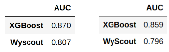
Figure 3. ROC-AUC value of our model and the Wyscout model on the training (left) and test (right) sets.
Consistently with the results obtained in the model analysis phase, we find that our algorithm gives a higher ROC-AUC value than the Wyscout xG model for the same dataset.
We see that the ROC-AUC value of our model on the test set is 1.3% lower than that obtained in the cross-validation on the training set, which may suggest that the model has not been able to generalize to unfamiliar data sets. However, we observe that the ROC-AUC value of the Wyscout model decreases by a similar percentage (1.4%) over the test set with respect to the training set.
Since the Wyscout model has not been trained on the same data set as our model, we conclude that this is not an overfitting problem. This is probably due to the fact that this dataset contains a high number of outliers, that is, clear scoring opportunities that are misses, or records of shots with a low a priori probability of conversion that end in a goal.
Next, we compare the ROC curves with one and the other model. This curve shows the true positive ratio (TPR) against the false positive ratio (FPR) by varying the value of the specific threshold to determine whether the predicted class is ‘Goal’ or ‘Miss’. The TPR and FPR values are defined as follows.


We see that the TPR measures the proportion of positives (goals) correctly predicted as such, and the FPR measures the proportion of negatives (misses) incorrectly predicted as a goal.
Thus, for a threshold equal to 0, all shots are predicted as ‘Goal’ since all probabilities exceed the threshold, so both TPR and FPR are equal to 1. At the other extreme, a threshold equal to 1 would result in predicting all shots as ‘Miss’ since the probability would be lower than the threshold in any case. This would result in a TPR and FPR equal to 0. A perfect classification consists of one for which the outcome of all observations is correctly predicted, so the TPR is equal to 1 (no false negatives) and the FPR is equal to 0 (no false positives).
Figure 4 shows the ROC curves of both xG models (our own and Wyscout’s), considering all thresholds from 0 to 1 in intervals of 0.01 to construct the ROC curve.
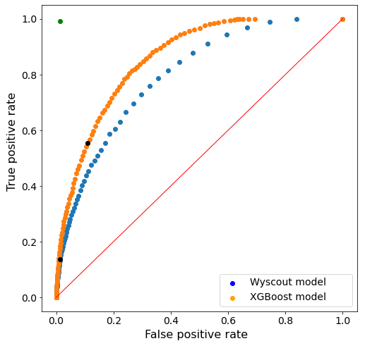
Figure 4. ROC curves obtained with the in-house model (orange) and the Wyscout model (blue). The black dots represent the results using the classification threshold of 0.5. For reference, the red line and green dot represent random classification and perfect classification, respectively.
As can be seen, the Wyscout model performs noticeably better than a random classification, since it is above the line joining the points (0,0) and (1,1). However, with our model a better ROC curve is obtained in that it is closer to the optimal (0,1) point, which would correspond to a perfect classification.
It is also observed that the classification results using the default threshold of 0.5 (represented by the black dots) differ greatly in both cases. In particular, we observe that the Wyscout model tends to underestimate the goal probabilities, resulting in a high number of false negatives (and thus a high TPR) compared to the number of false positives (low FPR). Our model, on the other hand, tends to predict higher probabilities, thus reducing the number of false negatives at the expense of increasing the number of false positives.
Figure 5 compares the confusion matrices obtained with one model and the other, which are constructed from the threshold of 0.5 explained above.
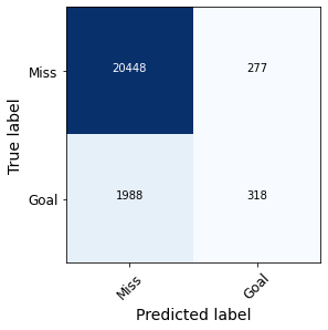
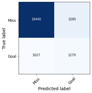
Figure 5. Confusion matrixes obtained with the Wyscout model (left) and our own model (right).
In fact, we observe that our model produces a considerably higher number of false positives than Wyscout’s model, while the number of false negatives decreases. Figure 6 compares the values of recall, precision and F1 metric for the ‘Goal’ class using one model and the other.
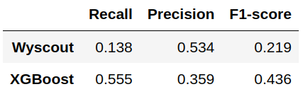
Figure 6. Comparison of recall, precision and F1-score of both models.
As we can see, precision is lower in our model due to the increase in false positives. However, the recall is much higher since the proportion of false negatives is drastically reduced in relation to the total number of positive observations. This makes the F1-score value, which is the harmonic mean of the two previous metrics, almost twice as high in our model as in the Wyscout model.
Conclusions and future work
As improvements to be made to the work, it is worth mentioning the possibility of testing new classification models or new combinations of hyperparameters for the models used. Also, different types of scaling or PCA could be used for each of the models proposed together with their corresponding grid search in each case. The possibilities of study are endless and this work represents only one way of approaching the problem.
Obviously, another possible point to improve would be the data ingestion, both in volume (which would favor the convergence of the models based on neural networks) and in variety (for example, having information such as the location of the players on the field at the time of the shot could undoubtedly improve the performance of our model).
Finally, a possible variation of this study would consist of generating a model that takes into account variables that we have not used here, such as specific information of the players or teams involved in the shot (accumulated statistics in the season or streaks of the shooting player, the opposing goalkeeper or both teams).
Although it would not be an xG metric as such, the results of this model would allow a more realistic assessment of the performance of a player or team in a given context (for example, it is not the same to face a mediocre goalkeeper as the best goalkeeper in the world). In this way, such metrics could be used to design specific game strategies for each player or match situation, and thus gain a great competitive advantage.
This is all! If you found this post interesting, we encourage you to visit the Data Science category to see all the related posts and to share it on your networks. See you soon!
