
In a previous article, we gave a theoretical introduction to Spark Structured Streaming where we analysed in depth the high-level API that Spark provides for processing massive real-time data streams (Structured Streaming). There, we looked at the essential theoretical concepts to understand how this API works, establishing a sufficient basis to be able to take a step forward towards a first practical implementation.
On this occasion, the aim is to provide a second contact with this interface from a practical point of view, presenting two simple examples that will allow the reader to have enough confidence to start implementing their first streaming data processing pipeline with Spark.
Sample data
In order to reinforce the theoretical concepts already seen in Structured Streaming, two practical examples will be presented in which we will try to condense all the essentials. For this purpose, two CSV files are provided which will contain the data that we will process in our practical examples:
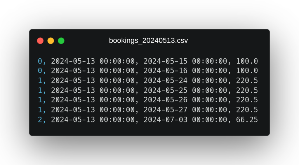
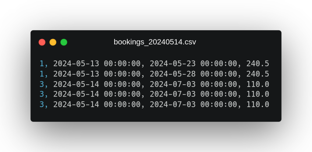
These files contain data on hotel bookings exploited by stay day, of which we have (in the order in which the fields appear in the file) their identifier, their booking date, the stay day and the price. As an additional note on this data, we can observe that in the second file a booking from the first file with identifier 1 reappears, which seems to have been modified by adding new days of stay.
Practical Example 1 – Base case without aggregations
From these example files, we propose as a practical case to develop a simple ETL that reads in streaming the files with this format that are deposited in a directory of the local file system, adds certain processed fields to them and writes the result in streaming in any sink. To deal with this scenario, the Scala code shown in the following image is proposed:
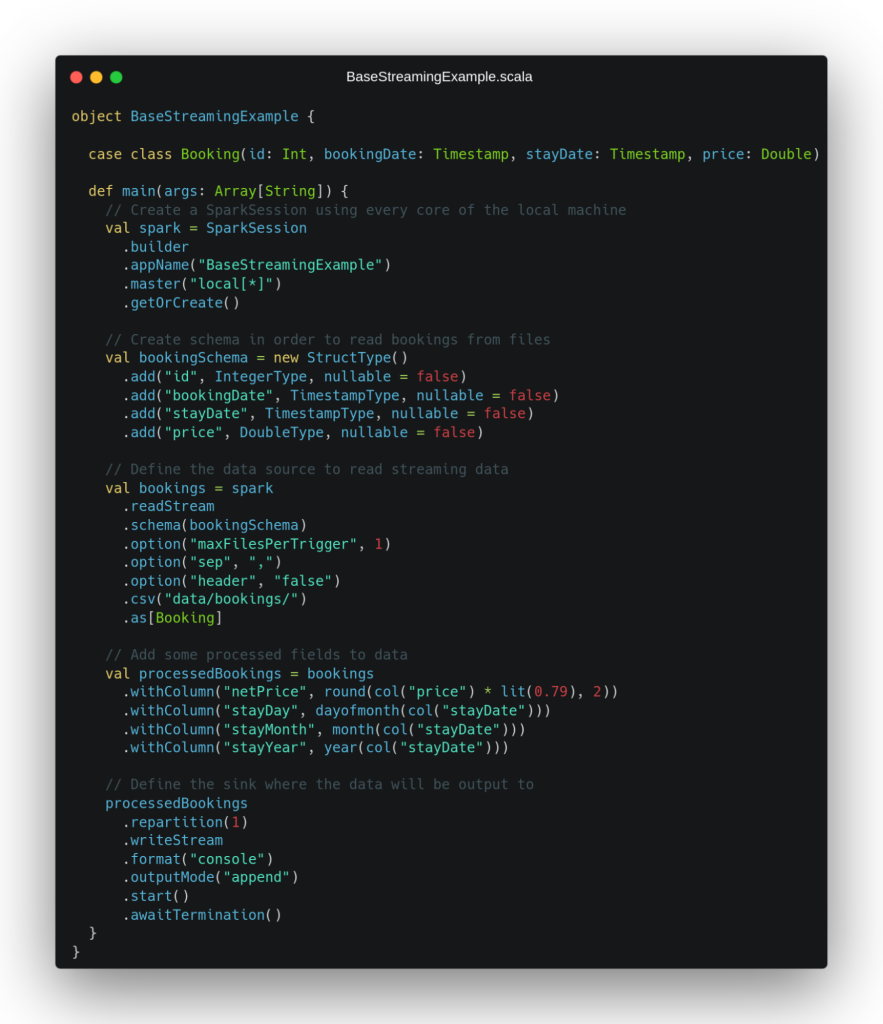
In this example, we can see how in the first lines we instantiate the Spark application and define the data schema that we will use to read from the CSV files. Then, we go on to establish the data source that will provide us with a data stream to process, which, as we have mentioned in this case, will be a file type data source. In the options we specify when defining this data source, we can see how a maxFilePerTrigger configuration is defined that will limit the number of files read per mini-batch when reading in streaming to 1.
This configuration has been defined for didactic reasons, so that the system considers both files given as input in different mini-batches of our streaming and, in this way, we can better see how the pipeline would behave in a real use case in which one file arrives later than the other. After defining the streaming data source, we proceed to perform some operations that add processed fields to the dataset obtained as input to the pipeline, adding the net price and some temporal fields extracted from the day of stay date.
Finally, we define the sink where we will write the data once it has been processed in streaming which, in this case (again for didactic purposes), will be a console output with the ‘append’ output mode. In the definition of this sink we can see that a repartition(1) statement is made in order to write a single file with all the processed data. When executing this code with the previously presented data, we obtain the following output by console:
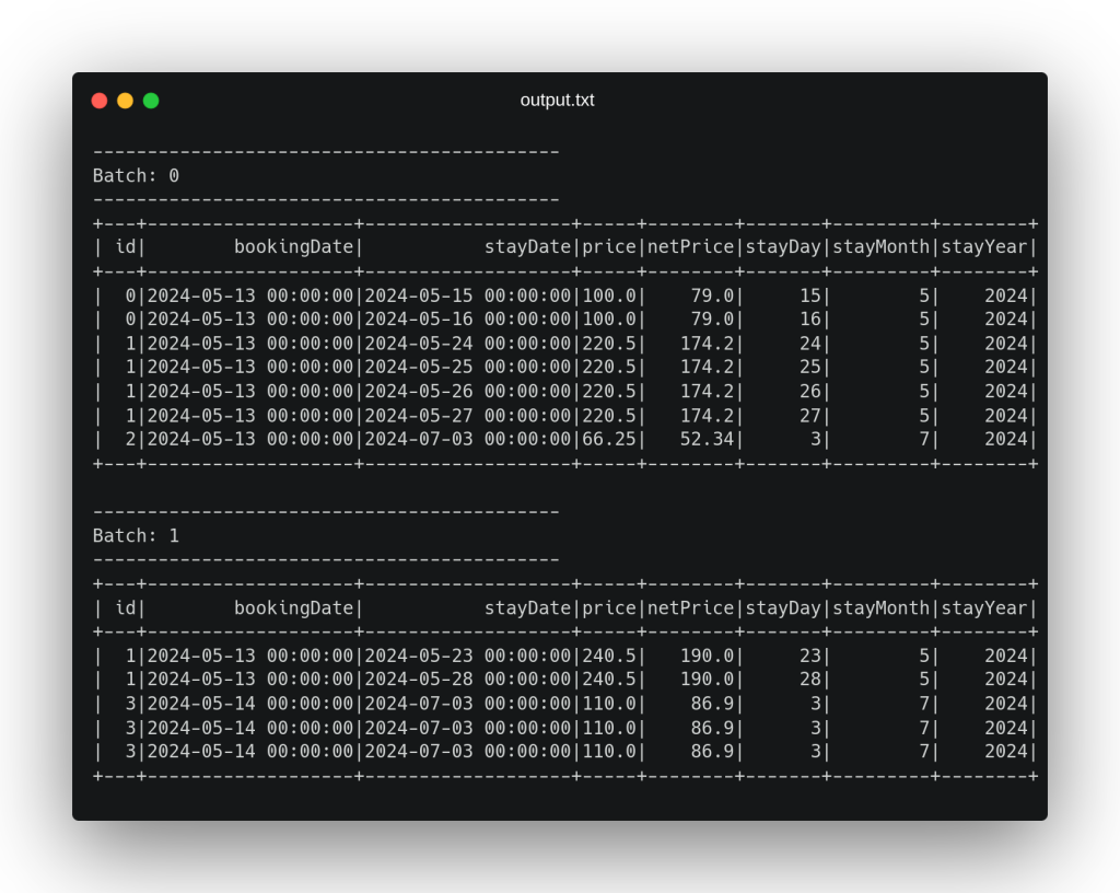
In this output we can see how each file has been considered in a different mini-batch, adding to each record the corresponding processed fields and emitting in the output a result record for each record received in streaming as input. After processing these two files, the pipeline waits to receive new files in the directory set as input path until the execution is finished externally, thanks to the last line of code .awaitTermination().
Practical Example 2 – More complex case with aggregations and internal state
After this first simple example, a more complex scenario is presented using the same input data. In this second case, we want to obtain the first stay day and the total price of each complete booking (considering the price of each of its stay days). For this, we will have to perform a grouping per booking, which we know implies having to store an internal state, which Spark will handle for us automatically. To solve this scenario, we propose the code in the following image:
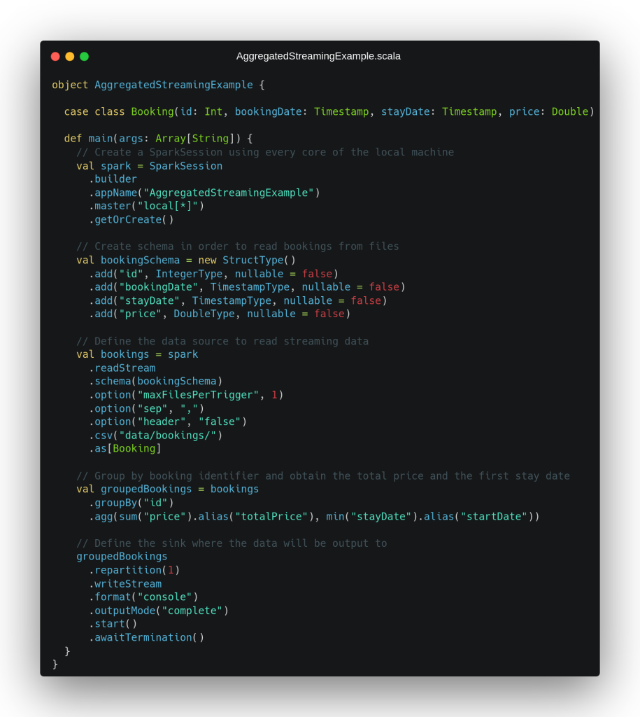
The first lines of this second scenario are identical to what we have seen in the previous example, including the definition of the streaming data source which has not changed since we still have the same input data. After this, we observe how the data is grouped by the booking identifier to, subsequently, obtain a sum of the price field for all the stay days and the first stay day in timestamp format by using the min operation.
After this process, we see the definition of the data sink, where it can be seen that the output mode has been changed to full mode, in order to produce as output all the reservations processed so far every time we receive new data, regardless of whether they have been changed, so that we can better observe what is happening underneath. When executing this code fragment, we get the following output on the screen:
As we can see in the output, when processing the first file, it is determined that the booking with identifier 1 has a total price of 882€ and a start date of 2024-05-24. Remember that in the second file there was an update of this reservation in which two more stay days were added, and, as we can see, when processing this second file, it has considered to calculate the aggregation both the data previously processed in the first file and the new updates that have arrived in the second file, increasing the total price to 1363€ and changing the start date.
This is because Spark has underneath stored an internal state of this aggregation to consider the previously processed data when new data arrives in our stream, thus obtaining the correct aggregation when considering all the data as a whole. Furthermore, if we look at the code, we can see that there is no reference to this internal state, since Spark takes care of it by defining an aggregation in the processing of our data.
Conclusion
In this post we have seen two simple case studies in which Spark is used to process a fictitious streaming dataset. In the first one, we have seen a simple scenario in which there are no aggregations in the data, only a simple processing is done to later write the continuous data stream somewhere else.
On the other hand, in the second example, a more complex use case has been seen, in which, as there are aggregations in the data, Spark is forced to store an internal representation of the previously aggregated data, returning consistent and robust results in a streaming context.
And that’s all! If you found this article interesting, we encourage you to visit the Data Engineering category to see all related posts and to share it on networks. See you soon!
