
In the field of Machine Learning there are multiple models whose internal structure makes it non-trivial to understand the why behind the decisions it makes. This set of models are widely known as black box models and are usually very powerful at detecting complex patterns in data. However, they exhibit behaviour that is not transparent to the user, such as neural networks.
Understanding in detail the reasons why a model has made a particular prediction or set of predictions is an increasingly demanded requirement in the world of artificial intelligence, especially when justifying such decisions is an insurmountable legal or corporate requirement due to important reasons such as discrimination of certain segments of the population.
It is in this context where different explainability techniques appear that allow us to shed light on the decisions made by our model, so that it is interpretable by any user, from the data scientist who has developed the model to the last stakeholder of the project.
In this post, we are going to see from a theoretical-practical point of view the use of an explainability technique that allows us to draw conclusions from a previously trained model, the SHAP values.
Types of explainability
This set of techniques aimed at the explainability of black box models can be classified according to several criteria. The first of these is whether or not the technique used depends on the machine learning model used. We will speak of agnostic techniques when these techniques are completely independent of the model used, and can be applied in any scenario. On the other hand, if the technique can only be used for a specific model or family of models, we will say that we are dealing with a model-specific technique.
Another useful classification to categorise these types of techniques is the distinction between local and global techniques. Local techniques are those that allow us to understand a prediction by our model of a particular instance, while global techniques are aimed at a more general understanding of the effect of different input features on the model’s output.
After introducing the concept of explainability and knowing the different types of techniques to interpret the output of black box models, we are going to look in detail at a specific explainability technique, the SHAP values.
SHAP values
SHAP values (SHapley Additive exPlanations) are a model-agnostic local explainability technique introduced in 2017 by Scott M. Lundberg and Su-In Lee in their paper ‘A Unified Approach to Interpreting Model Predictions’. These SHAP values come from game theory, specifically, from the theory behind measuring the impact of a subset of players (input features to our model) on the outcome of a cooperative game (the final prediction made by the model).
To calculate these SHAP values, we first select a particular instance or record in the data to be explained. These perturbations consist of variations of the original instance in which the value of one or several features has been replaced by a random value from the training dataset.
Subsequently, the elements of this new dataset are weighted using a complex methodology that gives more weight to those instances in which many or very few features have been perturbed, relying on game theory to quantify the value that these examples contribute to the final interpretation. Finally, a linear regression is fitted on this dataset using the prediction of our model as the target variable, obtaining a model whose coefficients allow us to understand the effect of each feature on the prediction of the chosen instance, which we call SHAP values.
Practical example
After explaining the theory behind these SHAP values, we are going to apply them to a real use case to understand a little better what they can provide us with in terms of explainability. For this, we have selected a dataset from Kaggle, Predict Online Gaming Behaviour Dataset, which captures various metrics and demographic data related to the behaviour of individuals in online video games. In it, a target variable indicating the degree to which the game retains the player is presented in order to analyse factors that may influence extreme dependence on video games.
For this practical example, some characteristics of the dataset were filtered and only those users with high or low retention were left to deal with the problem from a binary classification point of view, obtaining a dataset that was later divided into two independent datasets, one to train the model and the other to evaluate it. In the following image you can see the dataset before splitting it into two independent sets, consisting of a total of 20,658 different individuals and 7 characteristics plus the target variable high_engagement.
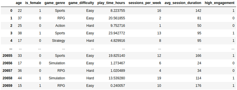
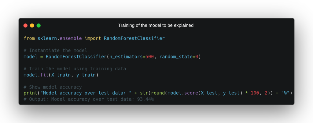
As we can see, in our data we have two categorical variables, game_genre and game_difficulty, which had to be transformed into a set of numerical variables by means of a One Hot Encoding in order to train a model that does not handle categorical variables. After this, a Random Forest composed of 500 weak estimators was instantiated and trained from this dataset, which obtained an accuracy of 93.44% on the evaluation dataset and will be the model whose explainability we will explore in detail through the use of the SHAP values.
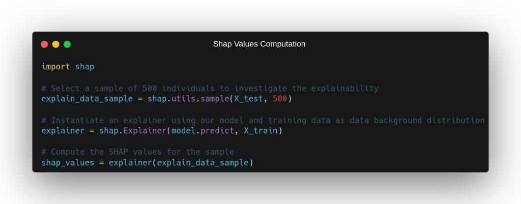
Once we have our target model trained, all that remains is to obtain and analyse the SHAP values for a set of instances to be explained. In the code of the following image you can see how we select a sample of 500 individuals to explain from the evaluation dataset, for which we calculate the SHAP values using the homonymous library. To obtain these SHAP values, it is necessary to define an explainer that knows the model method that generates the output predictions and a set of training data from which it will obtain the distribution of the data in order to create perturbations in the instance to be explained.
Using these calculated SHAP values, we are going to show several graphs that allow us to explain the behaviour of the model locally and globally. First, we select the first individual in our sample to explain, look at what the model has predicted and why it has made this prediction.
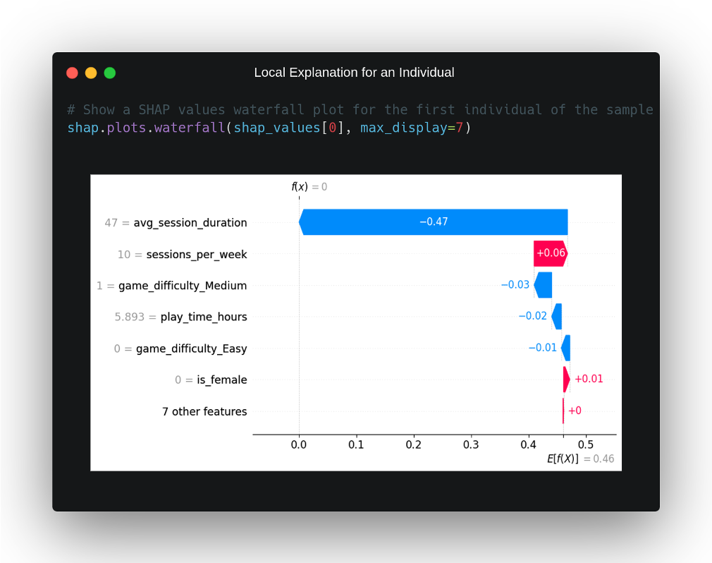
This particular instance belongs to an individual who does not have a high degree of retention by the online video game he plays and our model correctly predicts this from the input data. Why has he made this decision? In order to answer this question, we have to turn to the SHAP values that have been plotted for this instance in the waterfall plot above. In it, we can see on the X-axis the probability that the model determines that the individual belongs to the positive class, observing that, on average, this probability is 46%, which is normal considering that the dataset is quite balanced.
On the other hand, we can observe, in order of highest to lowest impact, those characteristics that have had the greatest weight in the model’s decision that this instance belongs to the negative class. Clearly, it can be seen that the model seems to have taken this decision for one feature in particular, the one that quantifies the average duration of the game session in minutes, and that takes a value well below the average of the dataset, with a time of 46 minutes per session for this individual with respect to the average of 99.43 minutes in the training dataset.
Behind this feature, we see that the second feature with the greatest impact on the model’s output provided output in the opposite direction, contributing to the model’s output, in this case, being in the positive class. This characteristic measures the number of playing sessions per week, and has a value in this individual of 10, which is slightly above the average of the training set. The impact of the other variables in this scenario is not very significant and, in general, does not seem to have influenced the output of the model very much.
Although SHAP values are considered as a local explainability technique, because by nature they must be calculated independently for each of the instances to be explained, it is possible to draw conclusions of global explainability by looking at the SHAP values of all the instances to be explained together. For this, the library offers us a graph called bee swarm that facilitates this task and which we can observe for the practical case in question in the following image:
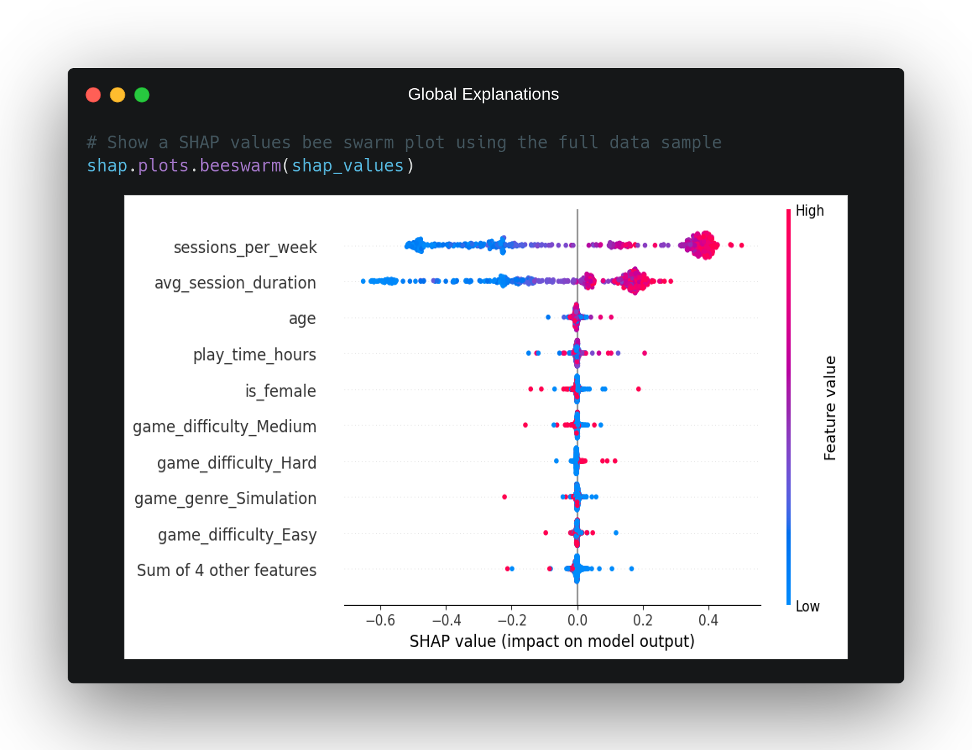
In this graph, we can see how on the X axis we have the impact on the model output of each characteristic, on the Y axis the characteristics that on average have had a greater impact on the model predictions and, finally, in a colour gradient from red to blue, we can observe for each point of the graph whether it corresponds to a high or low value of that variable. From this representation, we can draw a number of conclusions about the overall behaviour of the model:
- There are clearly two features that have a greater impact on the model’s output than the others, the number of gaming sessions per week,
sessions_per_week, and the average duration of those sessions in minutes,avg_session_duration. This is also supported by the local explanation above, where these two characteristics appeared to be the ones that determined the output for that individual. - If we look at the
sessions_per_weekvariable in isolation, we can see that, normally, high values of this variable correspond to an impact towards the positive class in the output of our model and vice versa. Moreover, this impact seems to be equal in both scenarios. It can also be observed that there are some cases where not excessively high values have had quite an impact on the model output, probably due to some interaction with some other variable. - The characteristic
avg_session_durationbehaves in a similar way tosessions_per_week, although with a significant difference: low values of this variable seem to have much more impact on the model output than high values, it is not as symmetrical in terms of its impact depending on the value. We even observe that, in certain scenarios, this variable has a greater negative impact than the first variable mentioned, despite the fact that, on average,sessions_per_weektends to have more impact on the output. - The third variable with the greatest impact is the individual’s age, although, as we can see, with a much lower average impact than the other two characteristics mentioned. The graph does not show clearly enough the impact of this variable depending on its values.
- As for the rest of the variables, they have very little impact on the output of the model in comparison in most scenarios, although it is true that there do seem to be isolated cases in which they have a non-negligible impact. For example, we can see that when the game has a high difficulty, there are several cases in which this difficulty has a positive impact on predicting positive class, indicating that a high difficulty can influence, in certain cases, high retention for an individual.
Conclusion
In this post, we have discussed an explainability technique for black box models called SHAP values, analysing how they are calculated and what conclusions they allow us to draw from the outputs of our model.
In addition, we have seen a simple case study in which these SHAP values have been used to analyse at a local and global level the explainability of a black box model, using different clear and intuitive graphs to draw effective conclusions.
And that’s all! If you found this article interesting, we encourage you to visit the Data Science category to see all the related posts and to share it on social networks. See you soon!
